Chapter 8 Analysis by Temporal Duration
Bar charts and tables to examine how contributions to conferences vary by methods
#spec(cpdata)

tempdata <- cpdata %>%
  select_if(is.numeric) %>%
  gather(key = Temporal, value = count, Hours:`Undefined Temporal`) %>%
  filter(count > 0) %>%
  group_by(`Temporal`) %>%
  summarise_all(sum, na.rm=T)

tfactor_order <- c('Hours', 'Days', 'Weeks', 'Months', 'Years', 'Decades', 'Centuries', 'Longer', 'Undefined Temporal')
tfactor_labels <- c('Hours', 'Days', 'Weeks', 'Months', 'Years', 'Decades', 'Centuries', 'Longer', 'Undefined')

tempdata <- tempdata %>%
  mutate(Temporal = factor(Temporal, levels = tfactor_order)) %>%
  arrange(Temporal)


utempdata <- cpdata %>%
  select_if(is.numeric) %>%
  gather(key = Temporal, value = count, Hours:Longer) %>%
  filter(count > 0) %>%
  group_by(`Temporal`) %>%
  summarise_all(sum, na.rm=T)

tfactor_order <- c('Hours', 'Days', 'Weeks', 'Months', 'Years', 'Decades', 'Centuries', 'Longer')
tfactor_labels <- c('Hours', 'Days', 'Weeks', 'Months', 'Years', 'Decades', 'Centuries', 'Longer')

utempdata <- utempdata %>%
  mutate(Temporal = factor(Temporal, levels = tfactor_order)) %>%
  arrange(Temporal)
8.1 Total Conference Contributions
General observations:
- Majority of studies do not define or report their temporal duration (65%)
- Those that do generally have durations longer than Years (~89%)
tempdata %>%
  select(Temporal, count) %>%
  mutate(prop = count/sum(count)) %>%
  mutate(prop = round(prop,3)) %>%
  kable() %>%
  kable_styling() %>%
scroll_box(width = "100%")| Temporal | count | prop |
|---|---|---|
| Days | 1 | 0.001 |
| Weeks | 3 | 0.004 |
| Months | 26 | 0.035 |
| Years | 74 | 0.099 |
| Decades | 123 | 0.164 |
| Centuries | 25 | 0.033 |
| Longer | 9 | 0.012 |
| Undefined Temporal | 487 | 0.651 |
ggplot(tempdata, aes(x=Temporal, y=count)) +
  geom_bar(stat="identity") +
  geom_text(aes(x=Temporal, y=max(count), label = paste0(round(100*count / sum(count),1), "%"), vjust=-0.5)) +
  ggtitle("All Data")+ theme(axis.text.x = element_text(angle = 15, hjust = 1)) +
  labs(y = "Abstract Count")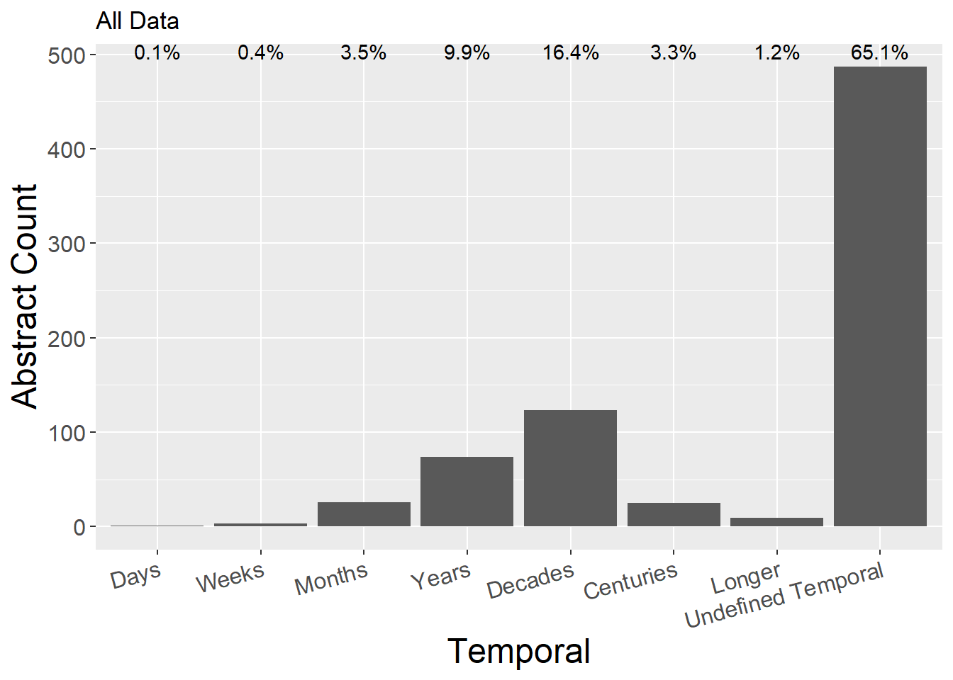
utempdata %>%
  select(Temporal, count) %>%
  mutate(prop = count/sum(count)) %>%
  mutate(prop = round(prop,3)) %>%
  kable() %>%
  kable_styling() %>%
scroll_box(width = "100%")| Temporal | count | prop |
|---|---|---|
| Days | 1 | 0.004 |
| Weeks | 3 | 0.011 |
| Months | 26 | 0.100 |
| Years | 74 | 0.284 |
| Decades | 123 | 0.471 |
| Centuries | 25 | 0.096 |
| Longer | 9 | 0.034 |
ggplot(utempdata, aes(x=Temporal, y=count)) +
  geom_bar(stat="identity") +
  geom_text(aes(x=Temporal, y=max(count), label = paste0(round(100*count / sum(count),1), "%"), vjust=-0.5)) +
  ggtitle("Excluding Undefined") +
  labs(y = "Abstract Count")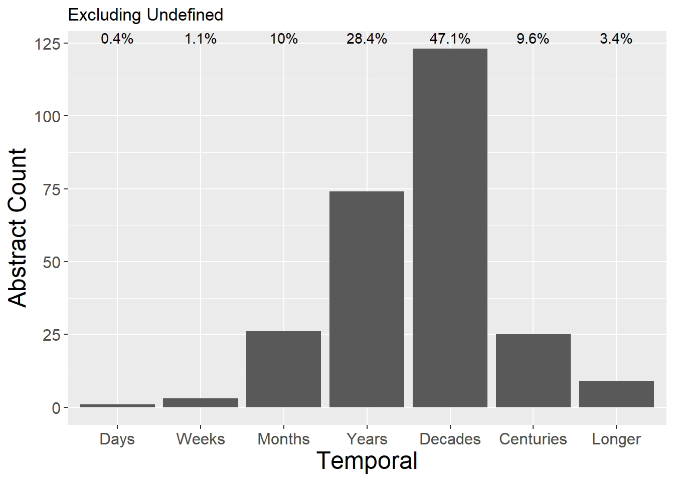
8.2 Author Affiliation
General observations:
- No obvious patterns
- Days, weeks and longer have very few responses (hence dominance)
authCounts <- tempdata %>%
  select(Temporal,Academic, Government,NGO,Business,Private) %>%
  mutate(sum = rowSums(.[2:6])) %>%   #calculate total for subsquent calcultation of proportion
  gather(key = Type, value = count, -Temporal, -sum) %>%
  mutate(prop = count / sum) #calculate proportion

authCountsW <- tempdata %>%
  select(Temporal,Academic, Government,NGO,Business,Private) %>%
  mutate(sum = rowSums(.[2:6])) %>%
  mutate_if(is.numeric, funs(prop = . / sum)) %>%
  mutate_at(8:12, round, 3)

ggplot(authCounts, aes(x=Temporal, y=count, fill=Type)) + geom_bar(stat="identity", colour="white") +
  scale_fill_viridis(discrete = TRUE) +
  theme(axis.text.x = element_text(angle = 30, hjust = 1)) +
  labs(fill="Affiliation", y = "Abstract Count", x="Temporal")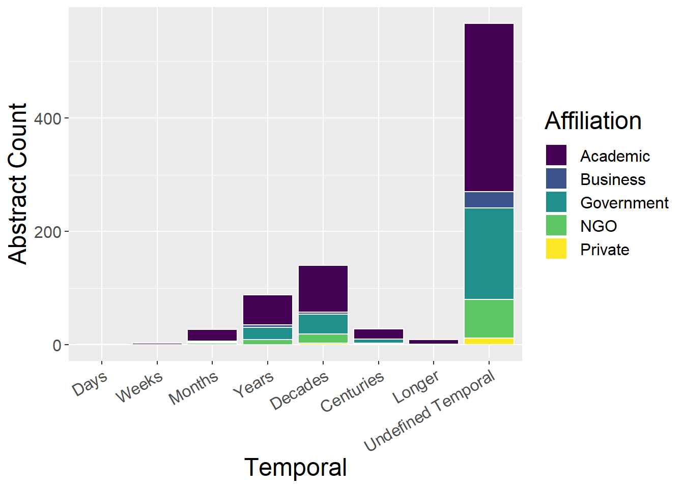
ggplot(authCounts, aes(x=Temporal, y=prop, fill=Type)) + geom_bar(stat="identity", colour="white") +
  scale_fill_viridis(discrete = TRUE) +
  theme(axis.text.x = element_text(angle = 30, hjust = 1)) +
  labs(fill="Affiliation", y = "Proportion", x="Temporal")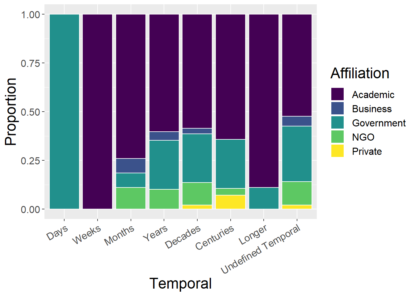
8.3 Landscape Type
8.3.1 Using all landscape types
General observations:
- Urban landscape studies tend to be shorter in duration
lspCounts <- tempdata %>%
  select(Temporal,`Upland rural`, `Lowland rural`, Urban,   Riverscape, Seascape, `Undefined LspType`,Other) %>%
  mutate(sum = rowSums(.[2:8])) %>%   #calculate total for subsquent calcultation of proportion
  gather(key = Type, value = count, -Temporal, -sum) %>%
  mutate(prop = count / sum)  #calculate proportion

ggplot(lspCounts, aes(x=Temporal, y=count, fill=Type)) + geom_bar(stat="identity", colour="white") +
  scale_fill_viridis(discrete = TRUE) +
  theme(axis.text.x = element_text(angle = 30, hjust = 1)) +
  labs(fill="Landscape", y = "Abstract Count", x="Temporal")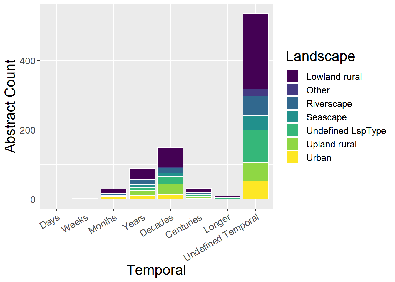
ggplot(lspCounts, aes(x=Temporal, y=prop, fill=Type)) + geom_bar(stat="identity", colour="white") +
  scale_fill_viridis(discrete = TRUE) +
  theme(axis.text.x = element_text(angle = 30, hjust = 1)) +
  labs(fill="Landscape", y = "Proportion", x="Temporal")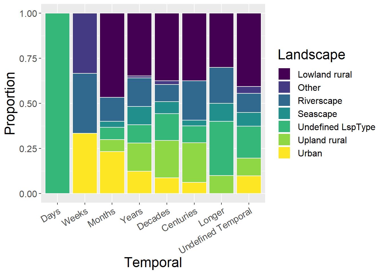
8.3.2 Without ‘Undefined LspType’ and ‘Other’ landscape types
General observations:
- Urban landscape studies tend to be shorter in duration
lspCounts <- tempdata %>%
  select(Temporal,`Upland rural`, `Lowland rural`, Urban,   Riverscape, Seascape) %>%
  mutate(sum = rowSums(.[2:6])) %>%   #calculate total for subsquent calcultation of proportion
  gather(key = Type, value = count, -Temporal, -sum) %>%
  mutate(prop = count / sum)  #calculate proportion

ggplot(lspCounts, aes(x=Temporal, y=count, fill=Type)) + geom_bar(stat="identity", colour="white") +
  scale_fill_viridis(discrete = TRUE) +
  theme(axis.text.x = element_text(angle = 30, hjust = 1)) +
  labs(fill="Landscape", y = "Abstract Count", x="Temporal")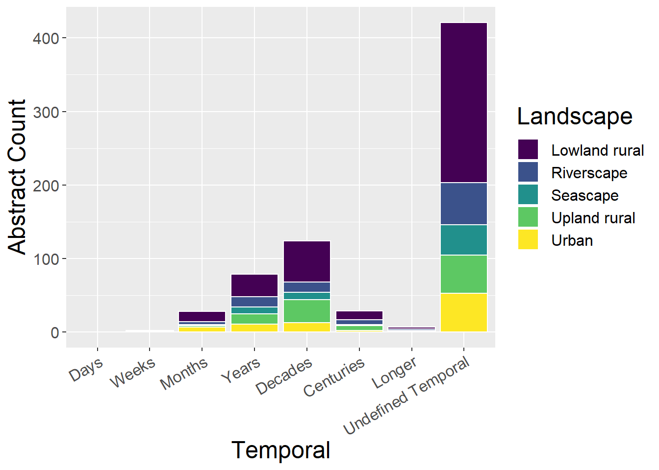
ggplot(lspCounts, aes(x=Temporal, y=prop, fill=Type)) + geom_bar(stat="identity", colour="white") +
  scale_fill_viridis(discrete = TRUE) +
  theme(axis.text.x = element_text(angle = 30, hjust = 1)) +
  labs(fill="Landscape", y = "Proportion", x="Temporal")
## Warning: Removed 5 rows containing missing values (position_stack).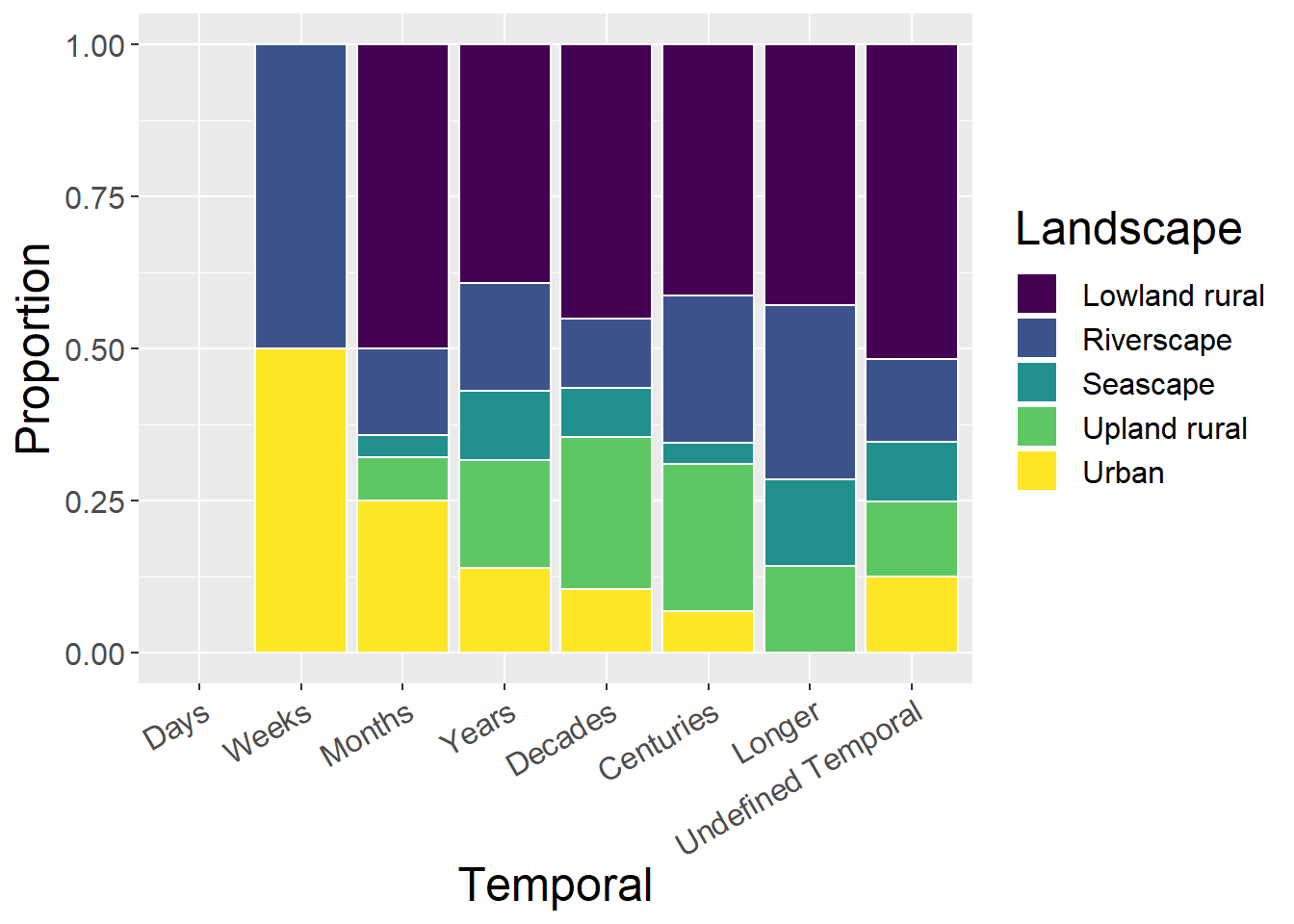
8.4 Organism
General observations
- Woodland and Forest have more studies at longer time extents
speciesCounts <- tempdata %>%
  select(Temporal, Mammals, Humans, Birds, Reptiles, Inverts, Plants, Amphibians, Fish, `Generic Habitat`,`Woodland Forests`) %>%
  mutate(sum = rowSums(.[2:11])) %>%   #calculate total for subsquent calcultation of proportion
  gather(key = Type, value = count, -Temporal, -sum) %>%
  mutate(prop = count / sum)  #calculate proportion

ggplot(speciesCounts, aes(x=Temporal, y=count, fill=Type)) + geom_bar(stat="identity", colour="white")  +
  scale_fill_viridis(discrete = TRUE) +
  theme(axis.text.x = element_text(angle = 30, hjust = 1)) +
  labs(fill="Organism", y = "Abstract Count", x="Temporal")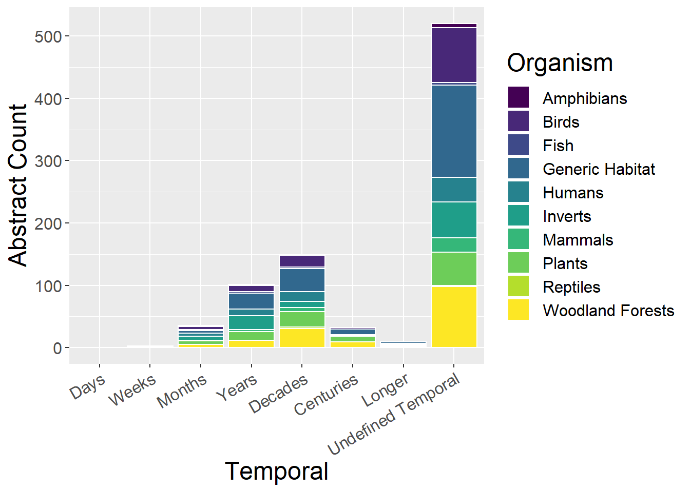
ggplot(speciesCounts, aes(x=Temporal, y=prop, fill=Type)) + geom_bar(stat="identity", colour="white")  +
  scale_fill_viridis(discrete = TRUE) +
  theme(axis.text.x = element_text(angle = 30, hjust = 1)) +
  labs(fill="Organism", y = "Proportion", x="Temporal")
## Warning: Removed 10 rows containing missing values (position_stack).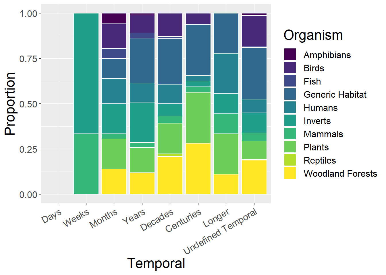
8.5 Methods
General observations:
- Theoretical studies seem to tend towards longer time extents
methodsCounts <- tempdata %>%
  select(Temporal, Empirical, Theoretical, Qualitative, Quantitative, GIS, `Remote sensing`) %>%
  mutate(sum = rowSums(.[2:7])) %>%
  gather(key = Type, value = count, -Temporal, -sum) %>%
  mutate(prop = count / sum)

ggplot(methodsCounts, aes(x=Temporal, y=count, fill=Type)) + geom_bar(stat="identity", colour="white") +
  scale_fill_viridis(discrete = TRUE) +
  theme(axis.text.x = element_text(angle = 30, hjust = 1)) +
  labs(fill="Method", y = "Abstract Count", x="Temporal")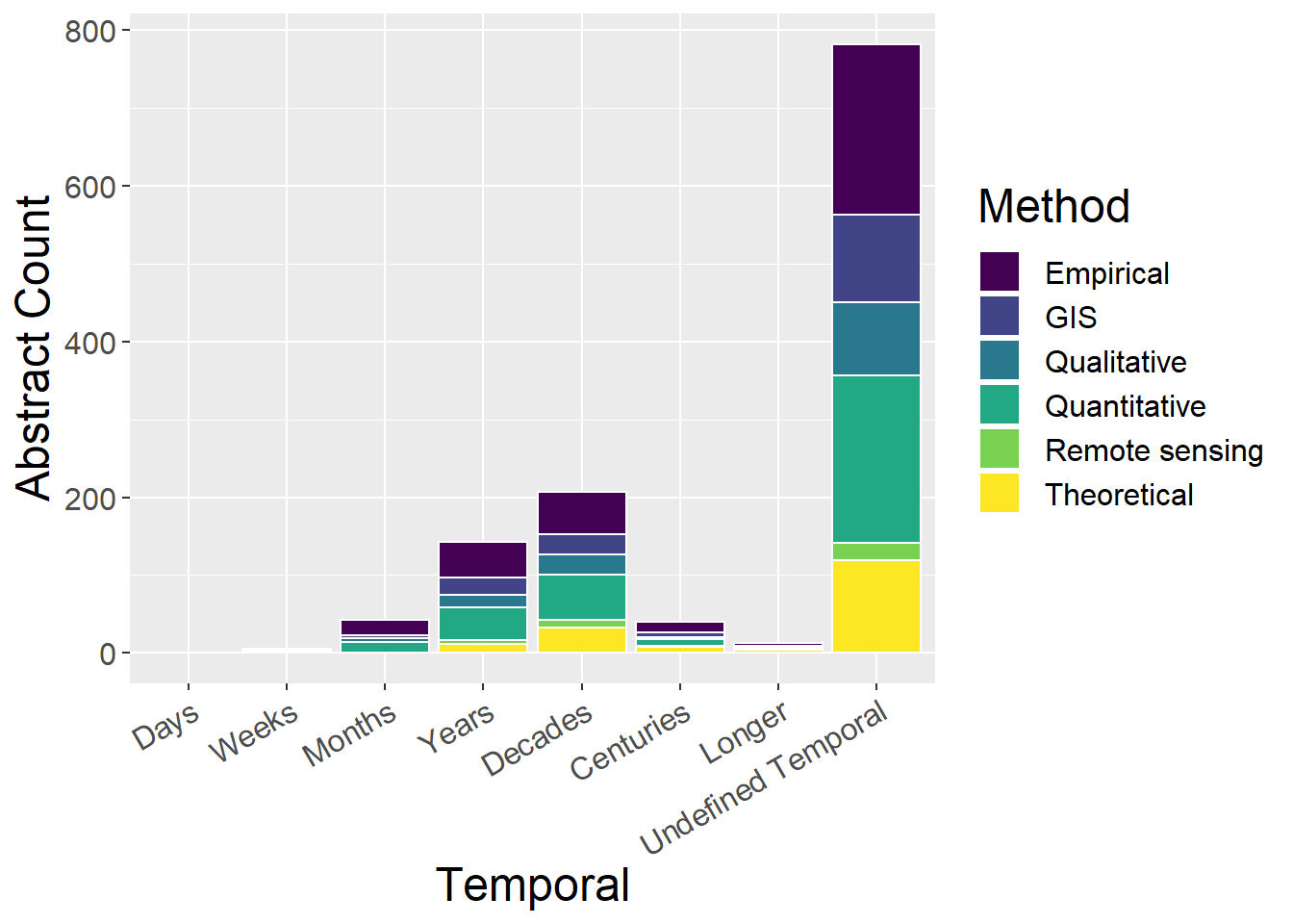
ggplot(methodsCounts, aes(x=Temporal, y=prop, fill=Type)) + geom_bar(stat="identity", colour="white") +
  scale_fill_viridis(discrete = TRUE) +
  theme(axis.text.x = element_text(angle = 30, hjust = 1)) +
  labs(fill="Method", y = "Proportion", x="Temporal")
## Warning: Removed 6 rows containing missing values (position_stack).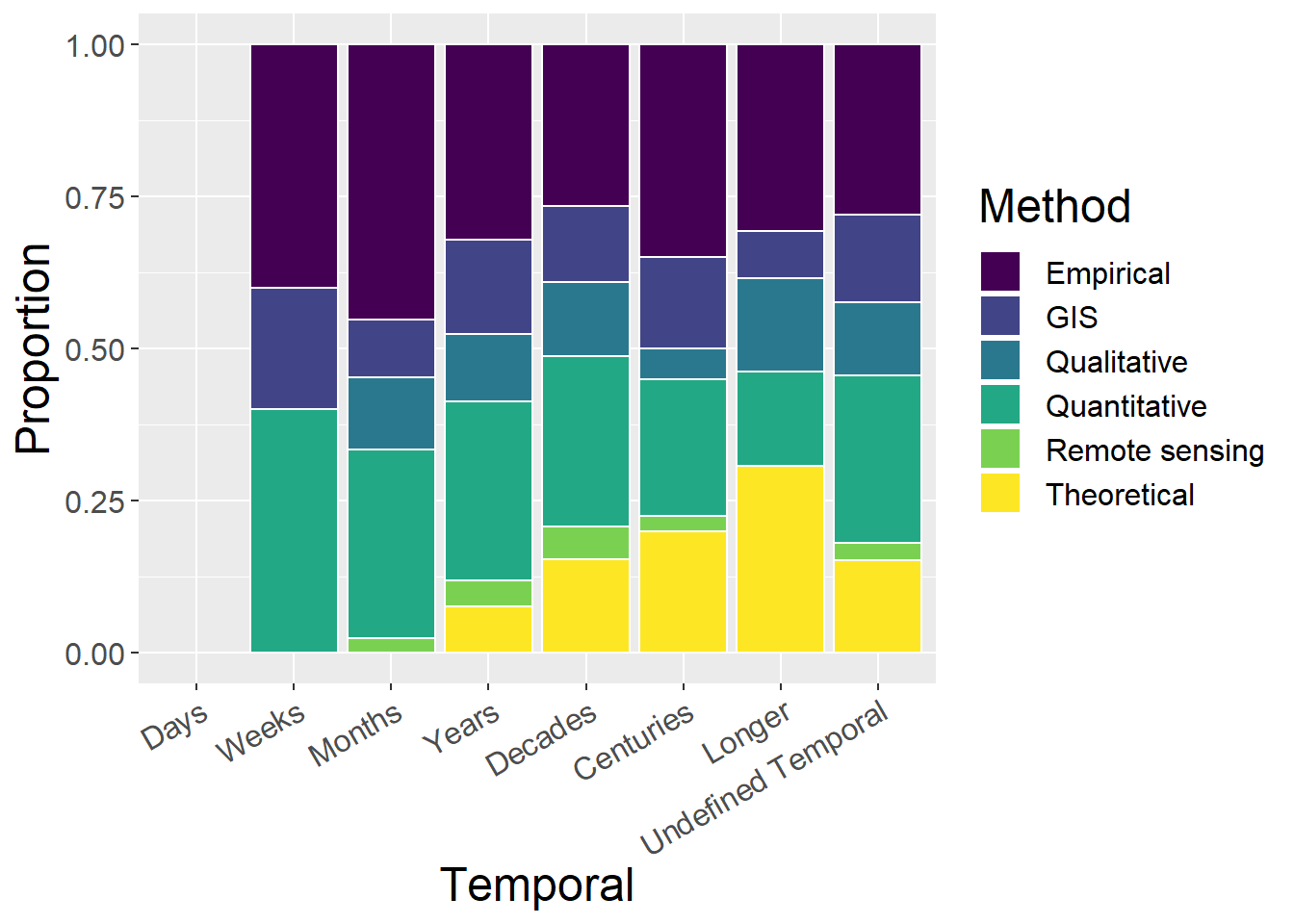
8.6 Spatial Extent
General observations:
- Continental studies tend to be over longer temporal extents
- Longer studies are less likely to have a defined spatial extent
- Shorter studies are more likely to have smaller spatial extent
extentCounts <- tempdata %>%
  select(Temporal, Micro, Mini, Local, Regional, National, Continental, Global,`Undefined Extent`) %>%
  mutate(sum = rowSums(.[2:9])) %>%
  gather(key = Type, value = count, -Temporal, -sum) %>%
  mutate(prop = count / sum)

factor_order <- c('Micro', 'Mini', 'Local', 'Regional', 'National', 'Continental', 'Global','Undefined Extent')
factor_labels <- c('Micro', 'Mini', 'Local', 'Regional', 'National', 'Continental', 'Global','Undefined')

ggplot(extentCounts, aes(x=Temporal, y=count, fill=factor(Type, level=factor_order))) + geom_bar(stat="identity", colour="white")  +
  scale_fill_viridis(discrete = TRUE) +
  theme(axis.text.x = element_text(angle = 30, hjust = 1)) +
  labs(fill="Spatial", y = "Abstract Count", x="Temporal")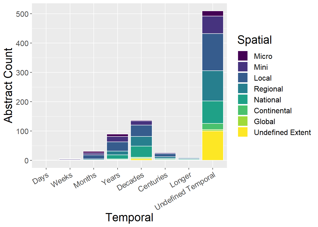
ggplot(extentCounts, aes(x=Temporal, y=prop, fill=factor(Type, level=factor_order))) + geom_bar(stat="identity", colour="white") +
  scale_fill_viridis(discrete = TRUE) +
  theme(axis.text.x = element_text(angle = 30, hjust = 1)) +
  labs(fill="Spatial", y = "Proportion", x="Temporal")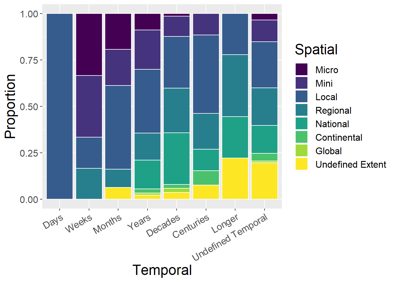
8.7 Concepts
General observations:
- Spatial Analysis tends towards shorter temporal extents
- Climate change studies seem to be longer extent studies
conceptCounts <- tempdata %>%
  select(Temporal, `PPS of landscapes`,
`Connectivity and fragmentation`, `Scale and scaling`,`Spatial analysis and modeling`,LUCC,`History and legacy`,`Climate change interactions`,`Ecosystem services`,`Landscape sustainability`,`Accuracy and uncertainty`
) %>%
  mutate(sum = rowSums(.[2:11])) %>%
  gather(key = Type, value = count, -Temporal, -sum) %>%
  mutate(prop = count / sum)

ggplot(conceptCounts, aes(x=Temporal, y=count, fill=Type)) + geom_bar(stat="identity", colour="white") +
  scale_fill_viridis(discrete = TRUE) +
  theme(axis.text.x = element_text(angle = 30, hjust = 1)) +
  labs(fill="Concept", y = "Abstract Count", x="Temporal")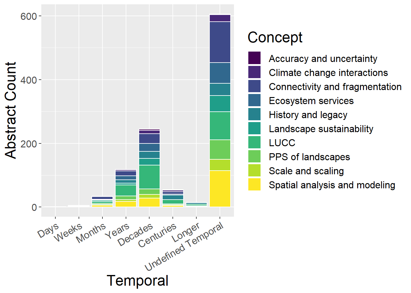
ggplot(conceptCounts, aes(x=Temporal, y=prop, fill=Type)) + geom_bar(stat="identity", colour="white") +
  scale_fill_viridis(discrete = TRUE) +
  theme(axis.text.x = element_text(angle = 30, hjust = 1)) +
  labs(fill="Concept", y = "Proportion", x="Temporal")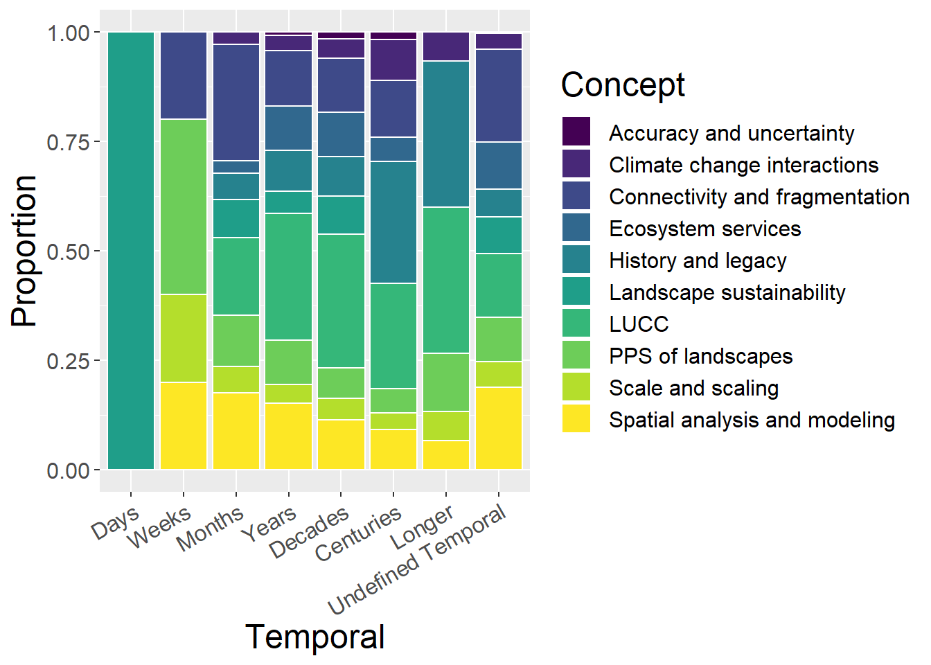
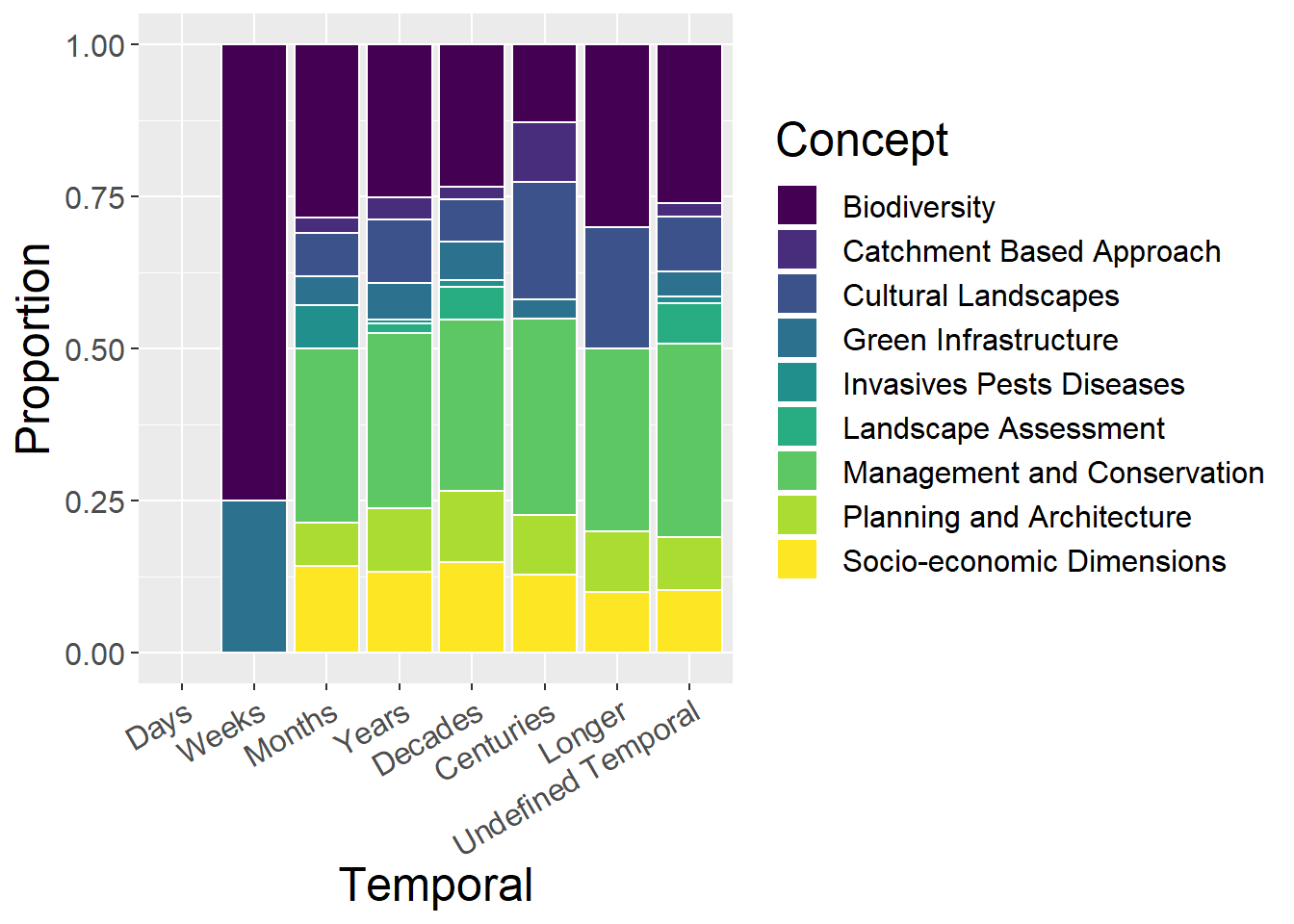
8.8 Other Concepts
General observations:
- No obvious patterns
otherCounts <- tempdata %>%
  select(Temporal, `Green Infrastructure`,`Planning and Architecture`,`Management and Conservation`,`Cultural Landscapes`,`Socio-economic Dimensions`,Biodiversity,`Landscape Assessment`,`Catchment Based Approach`,`Invasives Pests Diseases`
) %>%
  mutate(sum = rowSums(.[2:10])) %>%
  gather(key = Type, value = count, -Temporal, -sum) %>%
  mutate(prop = count / sum)

ggplot(otherCounts, aes(x=Temporal, y=count, fill=Type)) + geom_bar(stat="identity", colour="white") +
  scale_fill_viridis(discrete = TRUE) +
  theme(axis.text.x = element_text(angle = 30, hjust = 1)) +
  labs(fill="Concept", y = "Abstract Count", x="Temporal")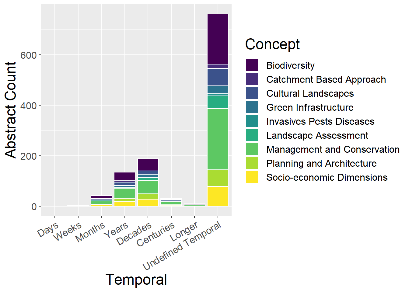
ggplot(otherCounts, aes(x=Temporal, y=prop, fill=Type)) + geom_bar(stat="identity", colour="white") +
  scale_fill_viridis(discrete = TRUE) +
  theme(axis.text.x = element_text(angle = 30, hjust = 1)) +
  labs(fill="Concept", y = "Proportion", x="Temporal")
## Warning: Removed 9 rows containing missing values (position_stack).