Chapter 2 Analysis by Conference Year

Bar charts and tables to examine how contributions to conferences have changed over time.

#Load Data
#After slightly cleaning column titles 

rm(list=ls())
library(tidyverse)
library(ggplot2)
library(kableExtra)
library(viridis)
path <- "C:/Users/k1076631/Google Drive/Research/Papers/InProgress/ialeUK_25years/QuantAnalysis/Rproject/"
filename <- "ialeUK25_abstracts_anon93.csv"
cpdata <- read_csv(paste0(path,filename))

this_theme <- theme_get() + 
  theme(legend.title = element_text(size=18),
        legend.text = element_text(size = 12),
        axis.title = element_text(size = 18), 
        axis.text = element_text(size = 12))
theme_set(this_theme)

#spec(cpdata)

yrdata <- cpdata %>%
  select_if(is.numeric) %>%
  group_by(`Conference Year`) %>%
  summarise_all(sum, na.rm=T) 

2.1 Total Conference Contributions

General observations:

• General increase through time to early 2000s then drop but steady through 2010s

summary <- cpdata %>%
  select_if(is.numeric) %>%
  group_by(`Conference Year`) %>%
  summarise_all(sum, na.rm=T) %>%
  select(`Conference Year`,Academic, Government,NGO,Business,Private) %>%
  mutate(count = rowSums(.[2:6])) %>%   
  select(`Conference Year`, count) %>%
  mutate(prop = count/sum(count)) %>%
  mutate(prop = round(prop,3)) 

summary %>%
  kable() %>%
  kable_styling() %>%
  scroll_box(width = "100%", height= "400px")

Conference Year	count	prop
1992	19	0.021
1993	12	0.013
1994	30	0.032
1995	44	0.048
1996	33	0.036
1997	62	0.067
1998	62	0.067
1999	33	0.036
2000	24	0.026
2001	58	0.063
2002	71	0.077
2004	66	0.071
2005	29	0.031
2006	58	0.063
2008	24	0.026
2009	33	0.036
2010	33	0.036
2011	46	0.050
2012	36	0.039
2014	40	0.043
2015	40	0.043
2016	27	0.029
2017	46	0.050

ggplot(summary, aes(x=`Conference Year`, y=count)) + 
  geom_bar(stat="identity") +
  labs(y = "Abstract Count") +
  scale_x_continuous(breaks = scales::pretty_breaks(n = 5))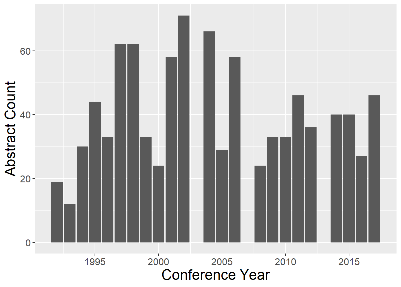

2.2 Author Affiliation

General observations:

• Academic contributors generally dominate
• Government contributors have decreased through time
• NGO attendance has replaced declines in Government?

authorCounts <- yrdata %>%
  select(`Conference Year`,Academic, Government,NGO,Business,Private) %>%
  mutate(yrsum = rowSums(.[2:6])) %>%   #calculate total for subsquent calcultation of proportion
  gather(key = Type, value = count, -`Conference Year`, -yrsum) %>%
  mutate(prop = count / yrsum)  #calculate proportion

yrdata %>%
  select(`Conference Year`,Academic, Government,NGO,Business,Private) %>%
  mutate(Total = rowSums(.[2:6])) %>%   #calculate total
  mutate_if(is.numeric, funs(prop = ./ Total)) %>%
  mutate_at(vars(ends_with("prop")), round, 3) %>% 
  select(-Total_prop) %>%
  kable() %>%
  kable_styling() %>%
  scroll_box(width = "100%", height= "400px")

## Warning: funs() is soft deprecated as of dplyr 0.8.0
## Please use a list of either functions or lambdas: 
## 
##   # Simple named list: 
##   list(mean = mean, median = median)
## 
##   # Auto named with `tibble::lst()`: 
##   tibble::lst(mean, median)
## 
##   # Using lambdas
##   list(~ mean(., trim = .2), ~ median(., na.rm = TRUE))
## This warning is displayed once per session.

Conference Year	Academic	Government	NGO	Business	Private	Total	Conference Year_prop	Academic_prop	Government_prop	NGO_prop	Business_prop	Private_prop
1992	6	12	0	1	0	19	104.842	0.316	0.632	0.000	0.053	0.000
1993	7	5	0	0	0	12	166.083	0.583	0.417	0.000	0.000	0.000
1994	11	15	2	1	1	30	66.467	0.367	0.500	0.067	0.033	0.033
1995	22	17	4	0	1	44	45.341	0.500	0.386	0.091	0.000	0.023
1996	16	15	2	0	0	33	60.485	0.485	0.455	0.061	0.000	0.000
1997	36	21	3	1	1	62	32.210	0.581	0.339	0.048	0.016	0.016
1998	39	21	2	0	0	62	32.226	0.629	0.339	0.032	0.000	0.000
1999	23	9	1	0	0	33	60.576	0.697	0.273	0.030	0.000	0.000
2000	15	8	1	0	0	24	83.333	0.625	0.333	0.042	0.000	0.000
2001	26	20	4	7	1	58	34.500	0.448	0.345	0.069	0.121	0.017
2002	38	16	15	1	1	71	28.197	0.535	0.225	0.211	0.014	0.014
2004	22	28	10	4	2	66	30.364	0.333	0.424	0.152	0.061	0.030
2005	19	6	4	0	0	29	69.138	0.655	0.207	0.138	0.000	0.000
2006	39	7	8	3	1	58	34.586	0.672	0.121	0.138	0.052	0.017
2008	18	3	2	1	0	24	83.667	0.750	0.125	0.083	0.042	0.000
2009	18	9	4	1	1	33	60.879	0.545	0.273	0.121	0.030	0.030
2010	19	3	11	0	0	33	60.909	0.576	0.091	0.333	0.000	0.000
2011	22	4	14	4	2	46	43.717	0.478	0.087	0.304	0.087	0.043
2012	23	5	7	1	0	36	55.889	0.639	0.139	0.194	0.028	0.000
2014	26	3	7	4	0	40	50.350	0.650	0.075	0.175	0.100	0.000
2015	20	8	6	6	0	40	50.375	0.500	0.200	0.150	0.150	0.000
2016	16	6	0	1	4	27	74.667	0.593	0.222	0.000	0.037	0.148
2017	30	7	4	3	2	46	43.848	0.652	0.152	0.087	0.065	0.043

ggplot(authorCounts, aes(x=`Conference Year`, y=count, fill=Type)) +
  geom_bar(stat="identity", colour="white") +
  scale_fill_viridis(discrete = TRUE) +
  labs(fill="Affiliation", y = "Abstract Count") +
  theme(legend.title = element_text(size=18),
        legend.text = element_text(size = 12),
        axis.title = element_text(size = 18), 
        axis.text = element_text(size = 12))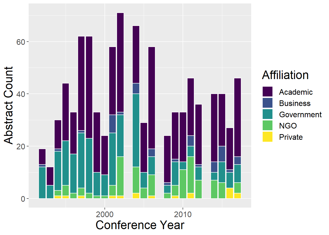 

ggplot(authorCounts, aes(x=`Conference Year`, y=prop, fill=Type)) + geom_bar(stat="identity", colour="white") +
  scale_fill_viridis(discrete = TRUE) +
  labs(fill="Affiliation", y = "Proportion") +
  scale_x_continuous(breaks = seq(1992, 2017, by = 2))+
  theme(axis.text.x = element_text(angle = 40, hjust = 1))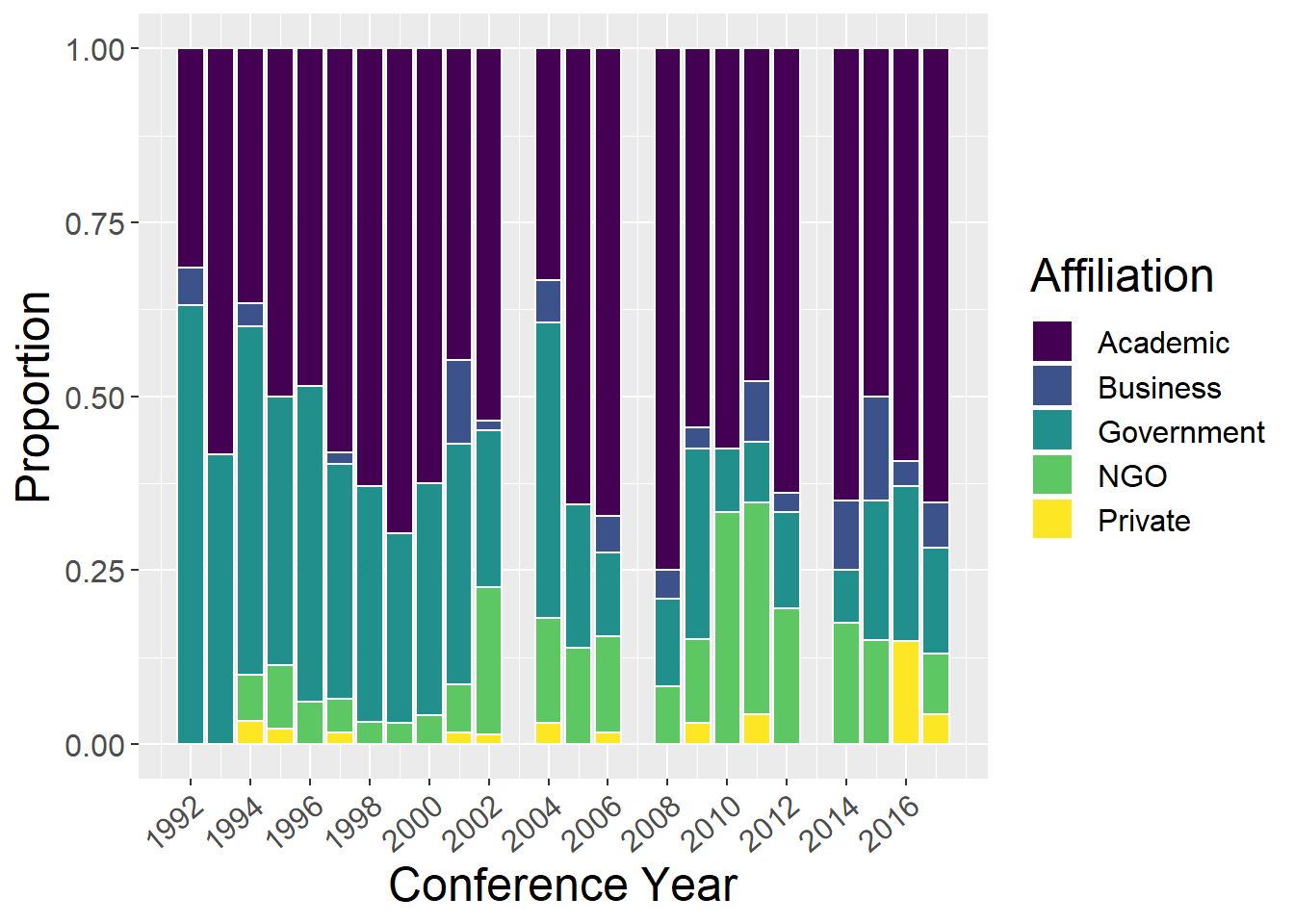 

2.3 Landscape Type

General observations:

• Lowland rural generaly dominates (but lesser contribution in later years)
• Spikes in some years for types (corresponding to special themes)
• Urban and Seascape both appear for first time in 1998; urban then constant presence, but seascape more variable until recent years

lspCounts <- yrdata %>%
  select(`Conference Year`,`Upland rural`, `Lowland rural`, Urban,  Riverscape, Seascape, `Undefined LspType`,Other) %>%
  mutate(yrsum = rowSums(.[2:8])) %>%
  gather(key = Type, value = count, -`Conference Year`, -yrsum) %>%
  mutate(prop = count / yrsum) 

yrdata %>%
  select(`Conference Year`,`Upland rural`, `Lowland rural`, Urban,  Riverscape, Seascape, `Undefined LspType`,Other) %>%
  mutate(Total = rowSums(.[2:8])) %>%
  mutate_if(is.numeric, funs(prop = ./ Total)) %>%
  mutate_at(vars(ends_with("prop")), round, 3) %>% 
  select(-Total_prop) %>%
  kable() %>%
  kable_styling() %>%
  scroll_box(width = "100%", height= "400px")

Conference Year	Upland rural	Lowland rural	Urban	Riverscape	Seascape	Undefined LspType	Other	Total	Conference Year_prop	Upland rural_prop	Lowland rural_prop	Urban_prop	Riverscape_prop	Seascape_prop	Undefined LspType_prop	Other_prop
1992	2	10	0	1	0	5	1	19	104.842	0.105	0.526	0.000	0.053	0.000	0.263	0.053
1993	7	8	0	1	1	2	3	22	90.591	0.318	0.364	0.000	0.045	0.045	0.091	0.136
1994	3	18	0	1	0	6	1	29	68.759	0.103	0.621	0.000	0.034	0.000	0.207	0.034
1995	5	11	0	0	2	15	2	35	57.000	0.143	0.314	0.000	0.000	0.057	0.429	0.057
1996	8	14	0	0	1	1	1	25	79.840	0.320	0.560	0.000	0.000	0.040	0.040	0.040
1997	10	31	0	4	0	4	3	52	38.404	0.192	0.596	0.000	0.077	0.000	0.077	0.058
1998	5	32	4	2	1	4	2	50	39.960	0.100	0.640	0.080	0.040	0.020	0.080	0.040
1999	7	23	4	4	1	7	3	49	40.796	0.143	0.469	0.082	0.082	0.020	0.143	0.061
2000	7	13	6	3	0	2	0	31	64.516	0.226	0.419	0.194	0.097	0.000	0.065	0.000
2001	6	32	3	0	0	9	1	51	39.235	0.118	0.627	0.059	0.000	0.000	0.176	0.020
2002	4	39	4	1	3	10	0	61	32.820	0.066	0.639	0.066	0.016	0.049	0.164	0.000
2004	7	32	2	1	0	13	5	60	33.400	0.117	0.533	0.033	0.017	0.000	0.217	0.083
2005	4	13	3	1	0	0	0	21	95.476	0.190	0.619	0.143	0.048	0.000	0.000	0.000
2006	0	7	3	47	0	0	1	58	34.586	0.000	0.121	0.052	0.810	0.000	0.000	0.017
2008	3	12	2	3	0	1	0	21	95.619	0.143	0.571	0.095	0.143	0.000	0.048	0.000
2009	0	10	2	4	0	10	0	26	77.269	0.000	0.385	0.077	0.154	0.000	0.385	0.000
2010	3	10	0	2	4	0	0	19	105.789	0.158	0.526	0.000	0.105	0.211	0.000	0.000
2011	6	10	6	7	1	10	1	41	49.049	0.146	0.244	0.146	0.171	0.024	0.244	0.024
2012	11	8	4	3	5	12	1	44	45.727	0.250	0.182	0.091	0.068	0.114	0.273	0.023
2014	0	5	38	6	2	1	0	52	38.731	0.000	0.096	0.731	0.115	0.038	0.019	0.000
2015	1	2	3	2	38	0	1	47	42.872	0.021	0.043	0.064	0.043	0.809	0.000	0.021
2016	7	8	4	1	4	12	0	36	56.000	0.194	0.222	0.111	0.028	0.111	0.333	0.000
2017	8	15	2	2	5	12	0	44	45.841	0.182	0.341	0.045	0.045	0.114	0.273	0.000

factor_order <- c('Upland rural', 'Lowland rural', 'Urban', 'Riverscape', 'Seascape', 'Undefined LspType','Other')
factor_labels <- c('Upland rural', 'Lowland rural', 'Urban',    'Riverscape', 'Seascape', 'Undefined','Other')

ggplot(lspCounts, aes(x=`Conference Year`, y=count, fill=factor(Type, level=factor_order))) + 
  geom_bar(stat="identity", colour="white") +
  scale_fill_viridis(discrete = TRUE, labels = factor_labels) +
  labs(fill="Lsp Type", y = "Abstract Count")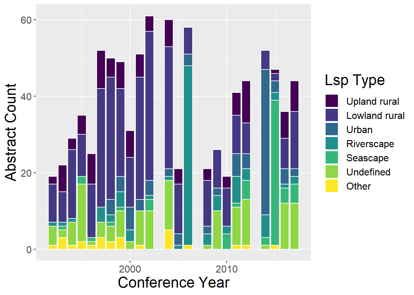

ggplot(lspCounts, aes(x=`Conference Year`, y=prop, fill=factor(Type, level=factor_order))) + 
  geom_bar(stat="identity", colour="white") +
  scale_fill_viridis(discrete = TRUE, labels = factor_labels) +
  labs(fill="Lsp Type", y = "Proportion") +
  scale_x_continuous(breaks = seq(1992, 2017, by = 2))+
  theme(axis.text.x = element_text(angle = 40, hjust = 1))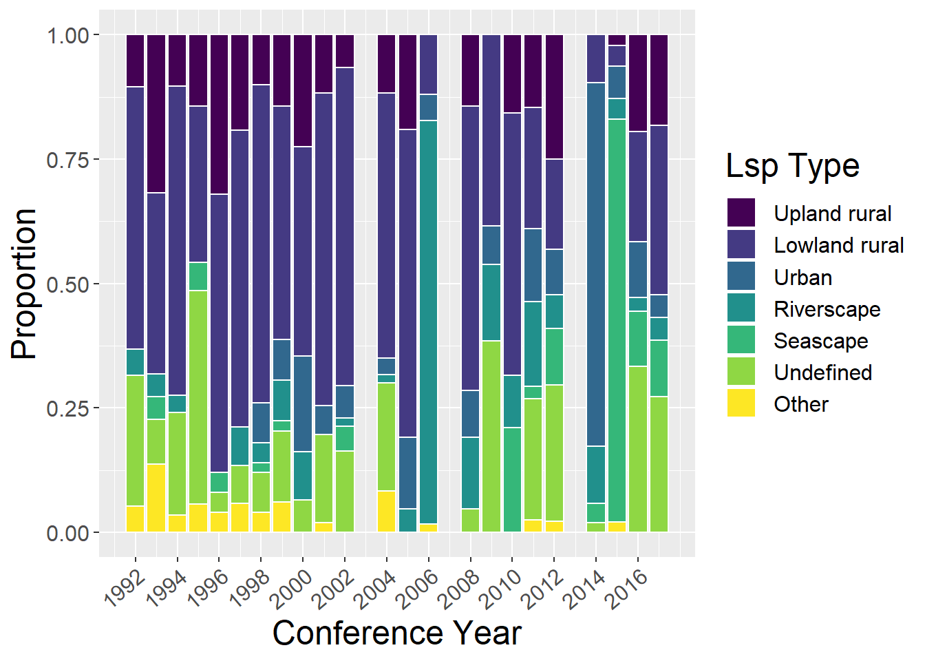 

2.4 Organism

General observations:

• No clear patterns
• Some years contain no Generic Habitat

sppCounts <- yrdata %>%
  select(`Conference Year`,Mammals, Humans, Birds, Reptiles, Inverts, Plants, Amphibians, Fish, `Generic Habitat`,`Woodland Forests`) %>%
  mutate(yrsum = rowSums(.[2:11])) %>%
  gather(key = Type, value = count, -`Conference Year`, -yrsum) %>%
  mutate(prop = count / yrsum) 

yrdata %>%
  select(`Conference Year`,Mammals, Humans, Birds, Reptiles, Inverts, Plants, Amphibians, Fish, `Generic Habitat`,`Woodland Forests`) %>%
  mutate(Total = rowSums(.[2:11])) %>%
  mutate_if(is.numeric, funs(prop = ./ Total)) %>%
  mutate_at(vars(ends_with("prop")), round, 3) %>% 
  select(-Total_prop) %>%
  kable() %>%
  kable_styling() %>%
  scroll_box(width = "100%", height= "400px")

Conference Year	Mammals	Humans	Birds	Reptiles	Inverts	Plants	Amphibians	Fish	Generic Habitat	Woodland Forests	Total	Conference Year_prop	Mammals_prop	Humans_prop	Birds_prop	Reptiles_prop	Inverts_prop	Plants_prop	Amphibians_prop	Fish_prop	Generic Habitat_prop	Woodland Forests_prop
1992	0	0	3	0	5	1	0	0	4	3	16	124.500	0.000	0.000	0.188	0.000	0.312	0.062	0.000	0.000	0.250	0.188
1993	1	3	1	1	0	1	1	0	9	3	20	99.650	0.050	0.150	0.050	0.050	0.000	0.050	0.050	0.000	0.450	0.150
1994	2	0	5	0	5	2	1	0	3	3	21	94.952	0.095	0.000	0.238	0.000	0.238	0.095	0.048	0.000	0.143	0.143
1995	2	0	2	0	5	3	1	0	9	6	28	71.250	0.071	0.000	0.071	0.000	0.179	0.107	0.036	0.000	0.321	0.214
1996	2	0	5	1	4	9	1	1	3	4	30	66.533	0.067	0.000	0.167	0.033	0.133	0.300	0.033	0.033	0.100	0.133
1997	1	0	5	0	14	23	1	0	5	3	52	38.404	0.019	0.000	0.096	0.000	0.269	0.442	0.019	0.000	0.096	0.058
1998	2	0	2	0	4	9	1	0	24	10	52	38.423	0.038	0.000	0.038	0.000	0.077	0.173	0.019	0.000	0.462	0.192
1999	4	0	4	0	7	3	1	0	20	8	47	42.532	0.085	0.000	0.085	0.000	0.149	0.064	0.021	0.000	0.426	0.170
2000	1	3	3	0	4	5	1	0	6	2	25	80.000	0.040	0.120	0.120	0.000	0.160	0.200	0.040	0.000	0.240	0.080
2001	3	0	7	1	7	15	0	0	29	5	67	29.866	0.045	0.000	0.104	0.015	0.104	0.224	0.000	0.000	0.433	0.075
2002	0	1	57	0	1	1	0	0	0	16	76	26.342	0.000	0.013	0.750	0.000	0.013	0.013	0.000	0.000	0.000	0.211
2004	7	0	8	0	9	8	0	0	1	47	80	25.050	0.088	0.000	0.100	0.000	0.112	0.100	0.000	0.000	0.012	0.588
2005	0	5	4	0	1	4	0	0	0	0	14	143.214	0.000	0.357	0.286	0.000	0.071	0.286	0.000	0.000	0.000	0.000
2006	1	2	2	0	12	5	2	1	25	1	51	39.333	0.020	0.039	0.039	0.000	0.235	0.098	0.039	0.020	0.490	0.020
2008	3	0	3	0	0	2	0	1	9	4	22	91.273	0.136	0.000	0.136	0.000	0.000	0.091	0.000	0.045	0.409	0.182
2009	3	0	1	0	2	0	0	1	7	7	21	95.667	0.143	0.000	0.048	0.000	0.095	0.000	0.000	0.048	0.333	0.333
2010	4	3	2	0	3	7	0	0	0	0	19	105.789	0.211	0.158	0.105	0.000	0.158	0.368	0.000	0.000	0.000	0.000
2011	1	0	3	0	4	3	0	0	0	3	14	143.643	0.071	0.000	0.214	0.000	0.286	0.214	0.000	0.000	0.000	0.214
2012	4	12	5	2	5	6	0	0	8	10	52	38.692	0.077	0.231	0.096	0.038	0.096	0.115	0.000	0.000	0.154	0.192
2014	1	9	0	0	3	3	1	2	23	3	45	44.756	0.022	0.200	0.000	0.000	0.067	0.067	0.022	0.044	0.511	0.067
2015	0	17	3	0	4	0	0	4	13	0	41	49.146	0.000	0.415	0.073	0.000	0.098	0.000	0.000	0.098	0.317	0.000
2016	0	11	0	0	2	0	0	0	20	0	33	61.091	0.000	0.333	0.000	0.000	0.061	0.000	0.000	0.000	0.606	0.000
2017	1	13	3	0	3	9	0	1	10	15	55	36.673	0.018	0.236	0.055	0.000	0.055	0.164	0.000	0.018	0.182	0.273

factor_order <- c('Amphibians', 'Birds', 'Fish','Woodland Forests','Generic Habitat', 'Humans','Inverts','Mammals','Plants','Reptiles')
factor_labels <- c('Amphibians', 'Birds', 'Fish','Forests','Generic Habitat', 'Humans','Inverts','Mammals','Plants','Reptiles')

ggplot(sppCounts, aes(x=`Conference Year`, y=count, fill=factor(Type, level=factor_order))) + 
  geom_bar(stat="identity", colour="white") +
  scale_fill_viridis(discrete = TRUE, labels = factor_labels) +
  labs(fill="Organism", y = "Abstract Count")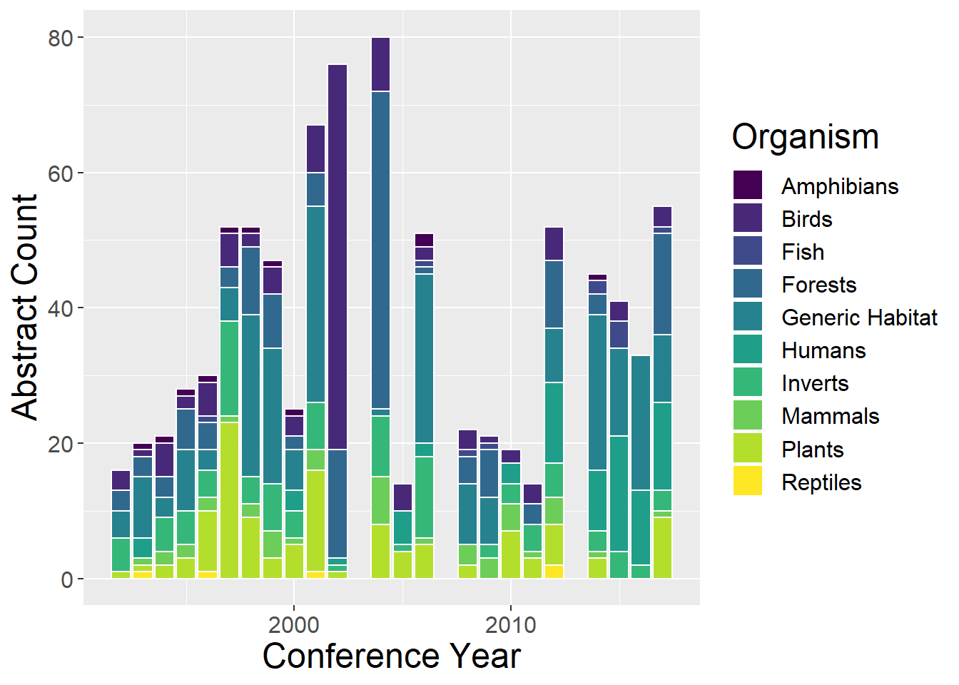

ggplot(sppCounts, aes(x=`Conference Year`, y=prop, fill=factor(Type, level=factor_order))) + 
  geom_bar(stat="identity", colour="white") +
  scale_fill_viridis(discrete = TRUE, labels = factor_labels) +
  labs(fill="Organism", y = "Proportion") +
  scale_x_continuous(breaks = seq(1992, 2017, by = 2))+
  theme(axis.text.x = element_text(angle = 40, hjust = 1))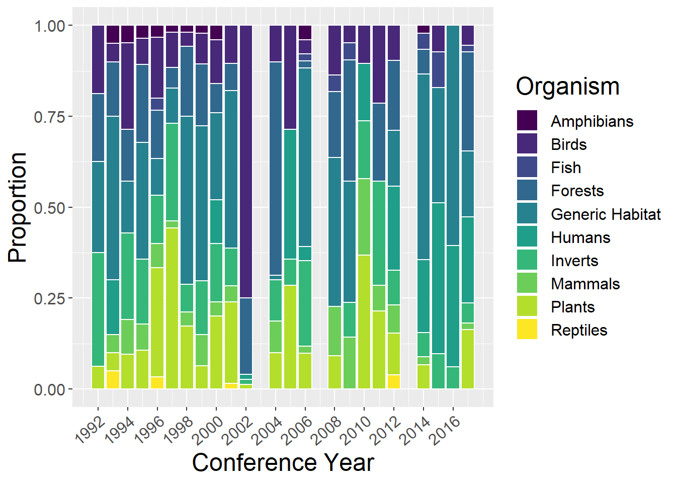 

2.5 Methods

General observations:

• Empirical studies have decreased through time
• GIS and qualitative have increased through time
• Quantitative and theoretical quite steady through time (although theoretical does seem to have reduced after initial years)

methodsCounts <- yrdata %>%
  select(`Conference Year`, Empirical, Theoretical, Qualitative, Quantitative, GIS, `Remote sensing`) %>%
  mutate(yrsum = rowSums(.[2:7])) %>%
  gather(key = Type, value = count, -`Conference Year`, -yrsum) %>%
  mutate(prop = count / yrsum) 

yrdata %>%
  select(`Conference Year`, Empirical, Theoretical, Qualitative, Quantitative, GIS, `Remote sensing`) %>%
  mutate(Total = rowSums(.[2:7])) %>%
  mutate_if(is.numeric, funs(prop = ./ Total)) %>%
  mutate_at(vars(ends_with("prop")), round, 3) %>% 
  select(-Total_prop) %>%
  kable() %>%
  kable_styling() %>%
  scroll_box(width = "100%", height= "400px")

Conference Year	Empirical	Theoretical	Qualitative	Quantitative	GIS	Remote sensing	Total	Conference Year_prop	Empirical_prop	Theoretical_prop	Qualitative_prop	Quantitative_prop	GIS_prop	Remote sensing_prop
1992	10	7	1	1	1	1	21	94.857	0.476	0.333	0.048	0.048	0.048	0.048
1993	1	0	9	7	0	1	18	110.722	0.056	0.000	0.500	0.389	0.000	0.056
1994	14	9	2	9	2	1	37	53.892	0.378	0.243	0.054	0.243	0.054	0.027
1995	15	13	2	9	4	1	44	45.341	0.341	0.295	0.045	0.205	0.091	0.023
1996	14	7	0	7	1	1	30	66.533	0.467	0.233	0.000	0.233	0.033	0.033
1997	40	2	0	1	12	0	55	36.309	0.727	0.036	0.000	0.018	0.218	0.000
1998	27	7	2	11	17	3	67	29.821	0.403	0.104	0.030	0.164	0.254	0.045
1999	25	11	2	24	10	6	78	25.628	0.321	0.141	0.026	0.308	0.128	0.077
2000	15	3	2	16	4	4	44	45.455	0.341	0.068	0.045	0.364	0.091	0.091
2001	36	5	11	32	2	1	87	23.000	0.414	0.057	0.126	0.368	0.023	0.011
2002	43	6	3	41	7	5	105	19.067	0.410	0.057	0.029	0.390	0.067	0.048
2004	35	25	13	46	12	0	131	15.298	0.267	0.191	0.099	0.351	0.092	0.000
2005	5	4	10	7	8	1	35	57.286	0.143	0.114	0.286	0.200	0.229	0.029
2006	23	6	7	18	14	1	69	29.072	0.333	0.087	0.101	0.261	0.203	0.014
2008	4	3	3	9	7	0	26	77.231	0.154	0.115	0.115	0.346	0.269	0.000
2009	9	8	6	6	10	0	39	51.513	0.231	0.205	0.154	0.154	0.256	0.000
2010	6	3	5	8	5	0	27	74.444	0.222	0.111	0.185	0.296	0.185	0.000
2011	9	7	9	12	7	0	44	45.705	0.205	0.159	0.205	0.273	0.159	0.000
2012	11	8	10	15	11	2	57	35.298	0.193	0.140	0.175	0.263	0.193	0.035
2014	6	10	14	23	13	4	70	28.771	0.086	0.143	0.200	0.329	0.186	0.057
2015	9	10	17	15	8	2	61	33.033	0.148	0.164	0.279	0.246	0.131	0.033
2016	5	7	14	13	14	2	55	36.655	0.091	0.127	0.255	0.236	0.255	0.036
2017	13	17	12	21	16	5	84	24.012	0.155	0.202	0.143	0.250	0.190	0.060

factor_order <- c('Empirical', 'GIS', 'Qualitative', 'Quantitative', 'Remote sensing', 'Theoretical')
factor_labels <- c('Empirical', 'GIS', 'Qualitative', 'Quantitative', 'RS', 'Theoretical')

ggplot(methodsCounts, aes(x=`Conference Year`, y=count, fill=factor(Type, level=factor_order)))  + 
  geom_bar(stat="identity", colour="white") +
  scale_fill_viridis(discrete = TRUE, labels = factor_labels) +
  labs(fill="Method", y = "Abstract Count")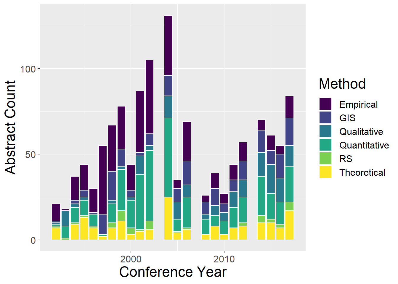

ggplot(methodsCounts, aes(x=`Conference Year`, y=prop, fill=factor(Type, level=factor_order))) + 
  geom_bar(stat="identity", colour="white") +
  scale_fill_viridis(discrete = TRUE, labels = factor_labels) +
  labs(fill="Method", y = "Proportion") +
  scale_x_continuous(breaks = seq(1992, 2017, by = 2))+
  theme(axis.text.x = element_text(angle = 40, hjust = 1))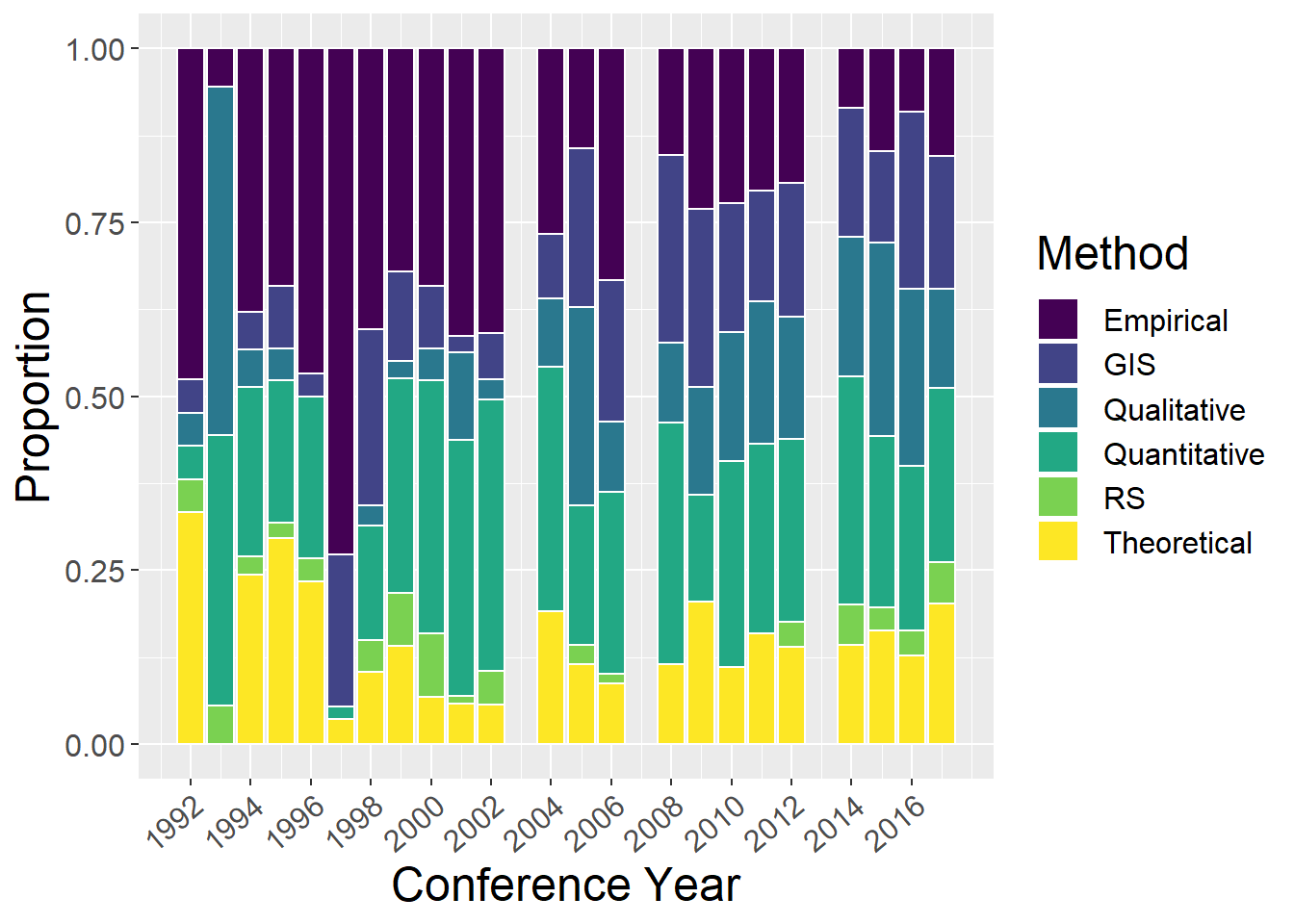 

2.6 Spatial Extent

General observations:

• Studies at ‘intermediate’ spatial extents dominate
• Global studies only appear from 2014 onwards

extentCounts <- yrdata %>%
  select(`Conference Year`, Micro, Mini, Local, Regional, National, Continental, Global,`Undefined Extent`) %>%
  mutate(yrsum = rowSums(.[2:9])) %>%
  gather(key = Type, value = count, -`Conference Year`, -yrsum) %>%
  mutate(prop = count / yrsum) 

yrdata %>%
  select(`Conference Year`, Micro, Mini, Local, Regional, National, Continental, Global,`Undefined Extent`) %>%
  mutate(Total = rowSums(.[2:9])) %>%
  mutate_if(is.numeric, funs(prop = ./ Total)) %>%
  mutate_at(vars(ends_with("prop")), round, 3) %>% 
  select(-Total_prop) %>%
  kable() %>%
  kable_styling() %>%
  scroll_box(width = "100%", height= "400px")

Conference Year	Micro	Mini	Local	Regional	National	Continental	Global	Undefined Extent	Total	Conference Year_prop	Micro_prop	Mini_prop	Local_prop	Regional_prop	National_prop	Continental_prop	Global_prop	Undefined Extent_prop
1992	0	6	3	0	7	1	0	2	19	104.842	0.000	0.316	0.158	0.000	0.368	0.053	0.000	0.105
1993	0	2	4	4	1	2	1	1	15	132.867	0.000	0.133	0.267	0.267	0.067	0.133	0.067	0.067
1994	2	7	6	9	1	2	0	3	30	66.467	0.067	0.233	0.200	0.300	0.033	0.067	0.000	0.100
1995	2	5	5	7	10	0	0	7	36	55.417	0.056	0.139	0.139	0.194	0.278	0.000	0.000	0.194
1996	2	5	8	3	8	0	0	1	27	73.926	0.074	0.185	0.296	0.111	0.296	0.000	0.000	0.037
1997	9	12	15	2	5	1	0	3	47	42.489	0.191	0.255	0.319	0.043	0.106	0.021	0.000	0.064
1998	3	4	21	12	6	2	0	6	54	37.000	0.056	0.074	0.389	0.222	0.111	0.037	0.000	0.111
1999	3	3	5	5	6	1	0	9	32	62.469	0.094	0.094	0.156	0.156	0.188	0.031	0.000	0.281
2000	2	4	2	8	3	0	0	2	21	95.238	0.095	0.190	0.095	0.381	0.143	0.000	0.000	0.095
2001	0	7	7	12	11	3	0	5	45	44.467	0.000	0.156	0.156	0.267	0.244	0.067	0.000	0.111
2002	1	7	17	11	6	3	0	11	56	35.750	0.018	0.125	0.304	0.196	0.107	0.054	0.000	0.196
2004	0	4	13	21	12	2	0	10	62	32.323	0.000	0.065	0.210	0.339	0.194	0.032	0.000	0.161
2005	3	1	10	6	6	1	0	0	27	74.259	0.111	0.037	0.370	0.222	0.222	0.037	0.000	0.000
2006	3	11	11	10	8	1	0	15	59	34.000	0.051	0.186	0.186	0.169	0.136	0.017	0.000	0.254
2008	0	0	9	6	3	1	0	0	19	105.684	0.000	0.000	0.474	0.316	0.158	0.053	0.000	0.000
2009	0	0	11	5	1	0	0	9	26	77.269	0.000	0.000	0.423	0.192	0.038	0.000	0.000	0.346
2010	0	1	3	6	6	1	0	0	17	118.235	0.000	0.059	0.176	0.353	0.353	0.059	0.000	0.000
2011	0	5	15	4	4	0	0	11	39	51.564	0.000	0.128	0.385	0.103	0.103	0.000	0.000	0.282
2012	0	4	9	15	8	1	0	2	39	51.590	0.000	0.103	0.231	0.385	0.205	0.026	0.000	0.051
2014	2	4	24	2	3	0	2	4	41	49.122	0.049	0.098	0.585	0.049	0.073	0.000	0.049	0.098
2015	1	2	10	8	8	1	2	7	39	51.667	0.026	0.051	0.256	0.205	0.205	0.026	0.051	0.179
2016	1	1	10	9	8	4	1	6	40	50.400	0.025	0.025	0.250	0.225	0.200	0.100	0.025	0.150
2017	2	6	17	7	16	2	3	1	54	37.352	0.037	0.111	0.315	0.130	0.296	0.037	0.056	0.019

factor_order <- c('Micro', 'Mini', 'Local', 'Regional', 'National', 'Continental', 'Global','Undefined Extent')
factor_labels <- c('Micro', 'Mini', 'Local', 'Regional', 'National', 'Continental', 'Global','Undefined')

ggplot(extentCounts, aes(x=`Conference Year`, y=count, fill=factor(Type, level=factor_order))) +
  geom_bar(stat="identity", colour="white") +
  scale_fill_viridis(discrete = TRUE, labels = factor_labels) +
  labs(fill="Spatial", y = "Abstract Count")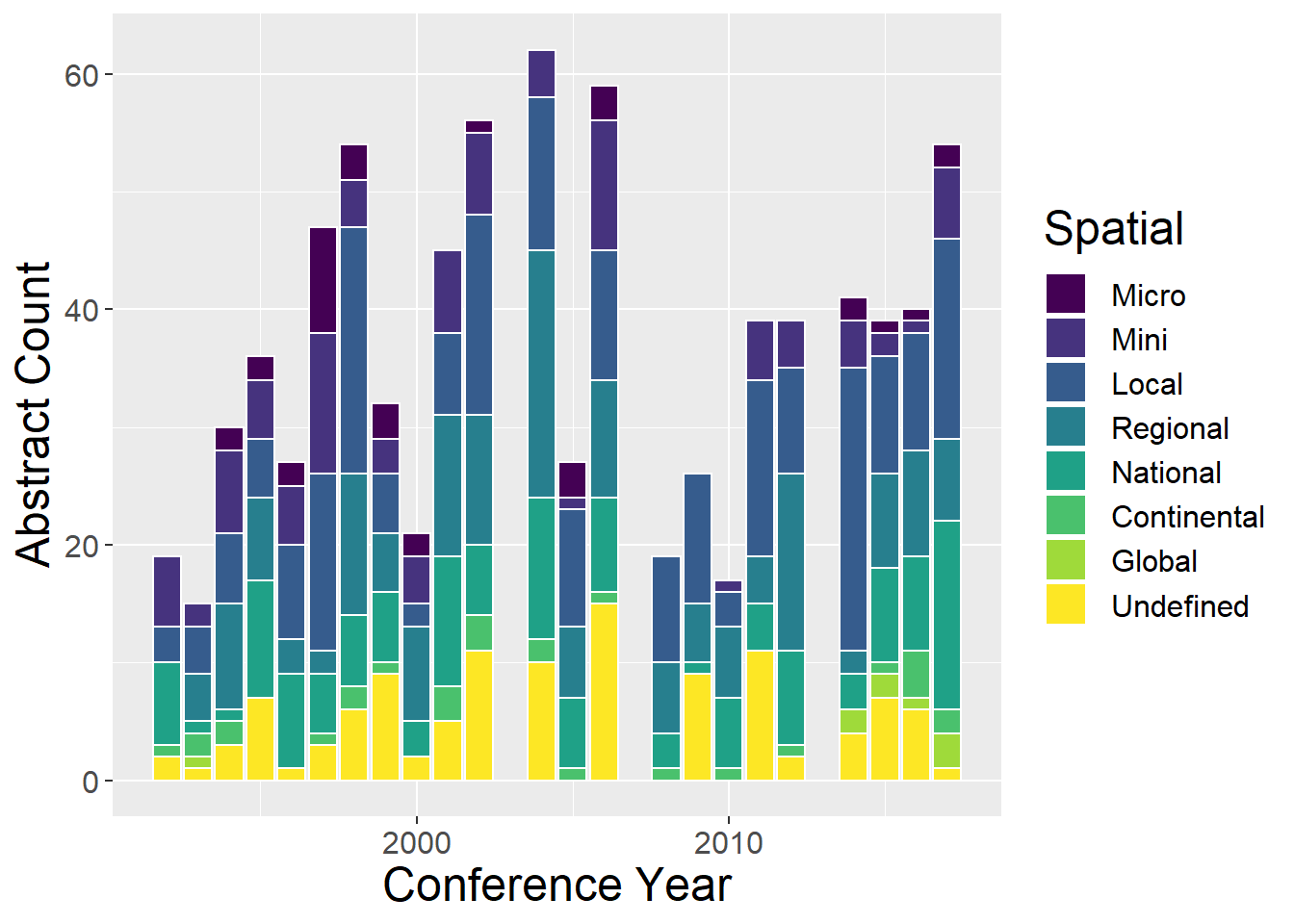

ggplot(extentCounts, aes(x=`Conference Year`, y=prop, fill=factor(Type, level=factor_order))) + 
  geom_bar(stat="identity", colour="white") +
  scale_fill_viridis(discrete = TRUE, labels = factor_labels) +
  labs(fill="Spatial", y = "Proportion") +
  scale_x_continuous(breaks = seq(1992, 2017, by = 2))+
  theme(axis.text.x = element_text(angle = 40, hjust = 1))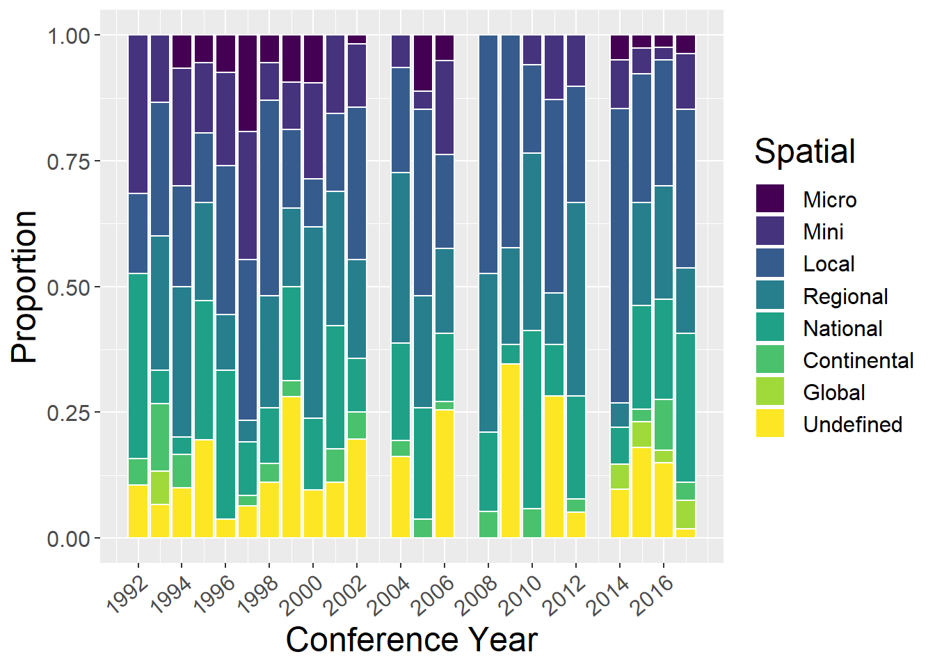 

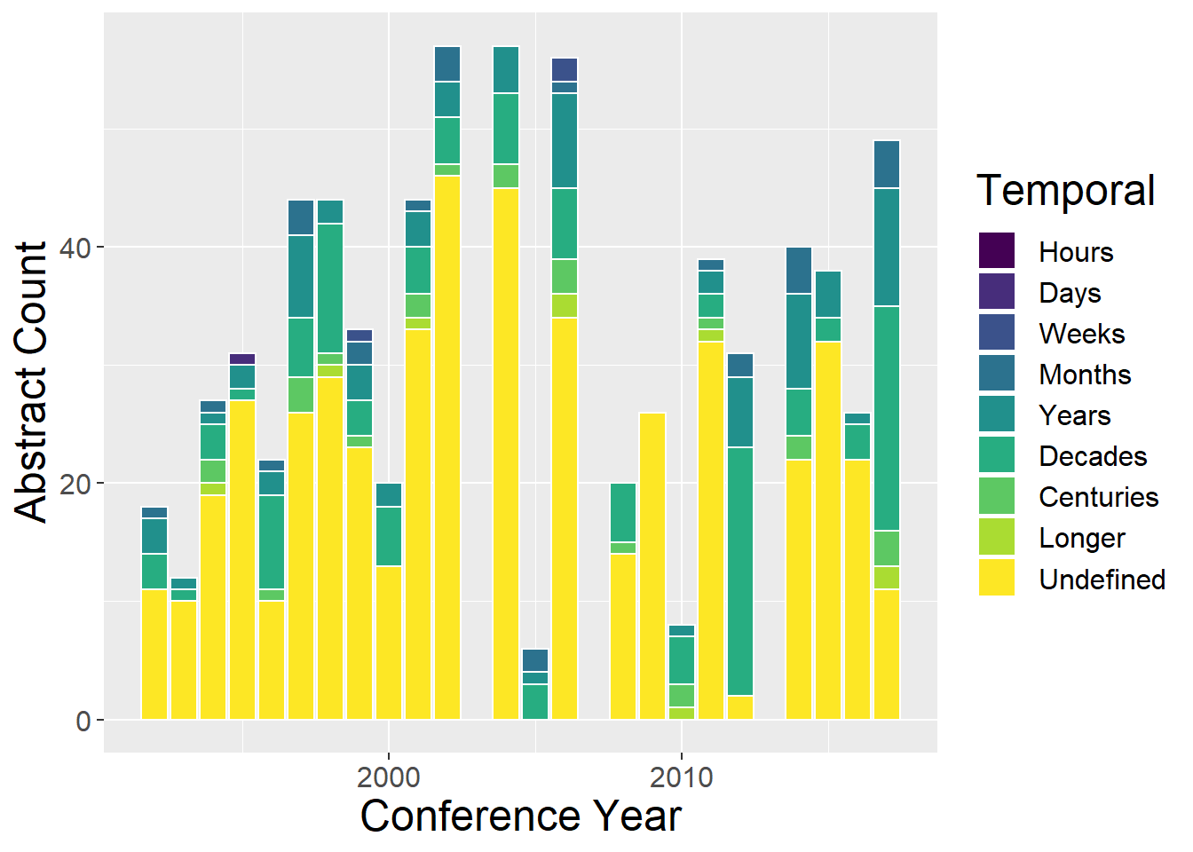
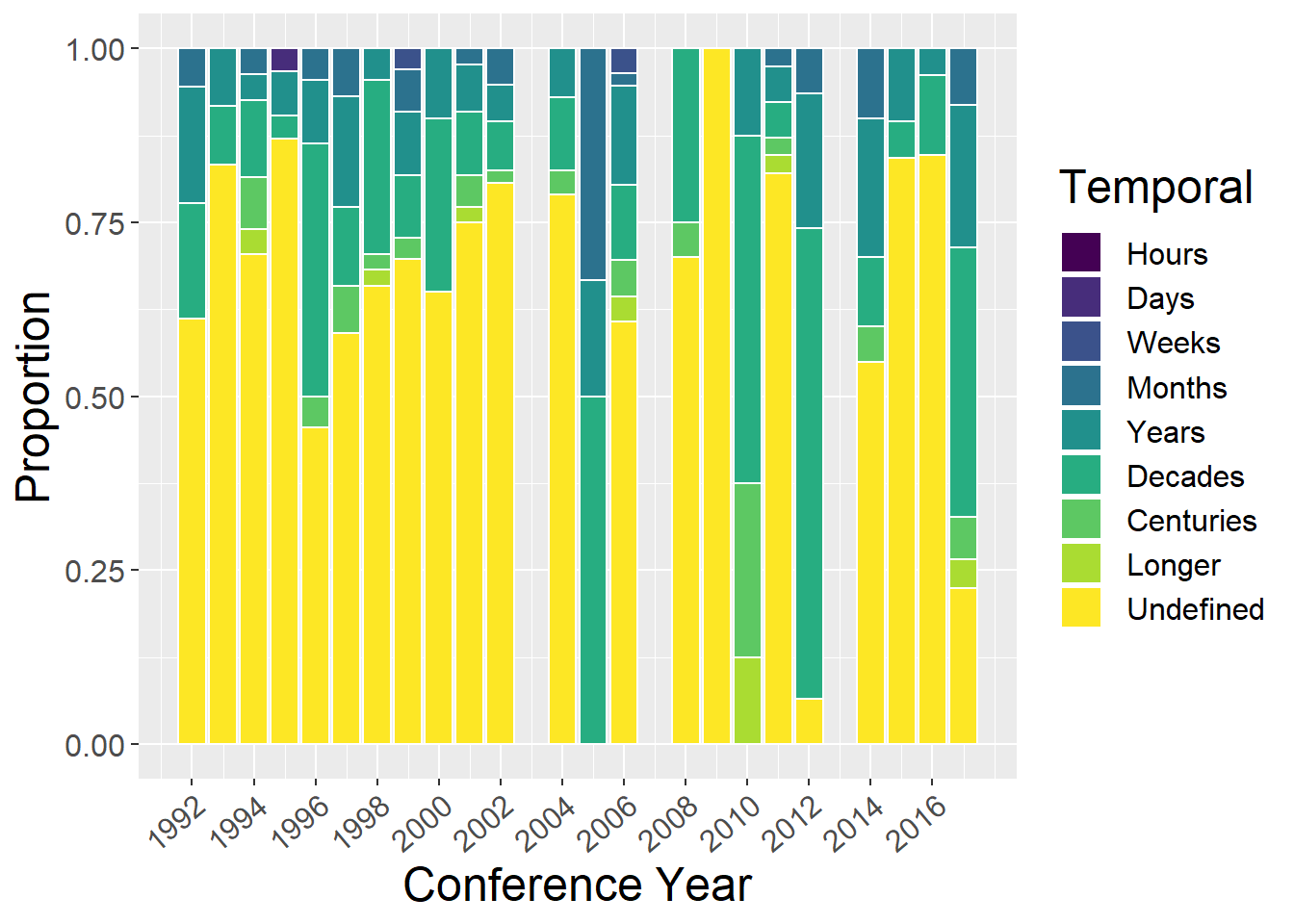
2.7 Temporal Extent

General observations:

• Most studies have undefined temporal duration
• Those that do are dominated by studies over decades and years

  Conference Year	Hours	Days	Weeks	Months	Years	Decades	Centuries	Longer	Undefined Temporal	Total	Conference Year_prop	Hours_prop	Days_prop	Weeks_prop	Months_prop	Years_prop	Decades_prop	Centuries_prop	Longer_prop	Undefined Temporal_prop
  1992	0	0	0	1	3	3	0	0	11	18	110.667	0	0.000	0.000	0.056	0.167	0.167	0.000	0.000	0.611
  1993	0	0	0	0	1	1	0	0	10	12	166.083	0	0.000	0.000	0.000	0.083	0.083	0.000	0.000	0.833
  1994	0	0	0	1	1	3	2	1	19	27	73.852	0	0.000	0.000	0.037	0.037	0.111	0.074	0.037	0.704
  1995	0	1	0	0	2	1	0	0	27	31	64.355	0	0.032	0.000	0.000	0.065	0.032	0.000	0.000	0.871
  1996	0	0	0	1	2	8	1	0	10	22	90.727	0	0.000	0.000	0.045	0.091	0.364	0.045	0.000	0.455
  1997	0	0	0	3	7	5	3	0	26	44	45.386	0	0.000	0.000	0.068	0.159	0.114	0.068	0.000	0.591
  1998	0	0	0	0	2	11	1	1	29	44	45.409	0	0.000	0.000	0.000	0.045	0.250	0.023	0.023	0.659
  1999	0	0	1	2	3	3	1	0	23	33	60.576	0	0.000	0.030	0.061	0.091	0.091	0.030	0.000	0.697
  2000	0	0	0	0	2	5	0	0	13	20	100.000	0	0.000	0.000	0.000	0.100	0.250	0.000	0.000	0.650
  2001	0	0	0	1	3	4	2	1	33	44	45.477	0	0.000	0.000	0.023	0.068	0.091	0.045	0.023	0.750
  2002	0	0	0	3	3	4	1	0	46	57	35.123	0	0.000	0.000	0.053	0.053	0.070	0.018	0.000	0.807
  2004	0	0	0	0	4	6	2	0	45	57	35.158	0	0.000	0.000	0.000	0.070	0.105	0.035	0.000	0.789
  2005	0	0	0	2	1	3	0	0	0	6	334.167	0	0.000	0.000	0.333	0.167	0.500	0.000	0.000	0.000
  2006	0	0	2	1	8	6	3	2	34	56	35.821	0	0.000	0.036	0.018	0.143	0.107	0.054	0.036	0.607
  2008	0	0	0	0	0	5	1	0	14	20	100.400	0	0.000	0.000	0.000	0.000	0.250	0.050	0.000	0.700
  2009	0	0	0	0	0	0	0	0	26	26	77.269	0	0.000	0.000	0.000	0.000	0.000	0.000	0.000	1.000
  2010	0	0	0	0	1	4	2	1	0	8	251.250	0	0.000	0.000	0.000	0.125	0.500	0.250	0.125	0.000
  2011	0	0	0	1	2	2	1	1	32	39	51.564	0	0.000	0.000	0.026	0.051	0.051	0.026	0.026	0.821
  2012	0	0	0	2	6	21	0	0	2	31	64.903	0	0.000	0.000	0.065	0.194	0.677	0.000	0.000	0.065
  2014	0	0	0	4	8	4	2	0	22	40	50.350	0	0.000	0.000	0.100	0.200	0.100	0.050	0.000	0.550
  2015	0	0	0	0	4	2	0	0	32	38	53.026	0	0.000	0.000	0.000	0.105	0.053	0.000	0.000	0.842
  2016	0	0	0	0	1	3	0	0	22	26	77.538	0	0.000	0.000	0.000	0.038	0.115	0.000	0.000	0.846
  2017	0	0	0	4	10	19	3	2	11	49	41.163	0	0.000	0.000	0.082	0.204	0.388	0.061	0.041	0.224

2.8 Concepts

General observations:

• Ecosystem services appear from 1998 and have grown recently
• Climate change interactions have only become common recently (since 2008)
• ‘Scale and scaling’ and ’connectivity and fragmentation seem to have decreased in recent years
• LUCC and Spatial Analysis are mainstays throughout

conceptCounts <- yrdata %>%
  select(`Conference Year`, `PPS of landscapes`,
`Connectivity and fragmentation`, `Scale and scaling`,`Spatial analysis and modeling`,LUCC,`History and legacy`,`Climate change interactions`,`Ecosystem services`,`Landscape sustainability`,`Accuracy and uncertainty`
) %>%
  mutate(yrsum = rowSums(.[2:11])) %>%
  gather(key = Type, value = count, -`Conference Year`, -yrsum) %>%
  mutate(prop = count / yrsum) 

yrdata %>%
  select(`Conference Year`, `PPS of landscapes`,
`Connectivity and fragmentation`, `Scale and scaling`,`Spatial analysis and modeling`,LUCC,`History and legacy`,`Climate change interactions`,`Ecosystem services`,`Landscape sustainability`,`Accuracy and uncertainty`
) %>%
  mutate(Total = rowSums(.[2:11])) %>%
  mutate_if(is.numeric, funs(prop = ./ Total)) %>%
  mutate_at(vars(ends_with("prop")), round, 3) %>% 
  select(-Total_prop) %>%
  kable() %>%
  kable_styling() %>%
  scroll_box(width = "100%", height= "400px")

Conference Year	PPS of landscapes	Connectivity and fragmentation	Scale and scaling	Spatial analysis and modeling	LUCC	History and legacy	Climate change interactions	Ecosystem services	Landscape sustainability	Accuracy and uncertainty	Total	Conference Year_prop	PPS of landscapes_prop	Connectivity and fragmentation_prop	Scale and scaling_prop	Spatial analysis and modeling_prop	LUCC_prop	History and legacy_prop	Climate change interactions_prop	Ecosystem services_prop	Landscape sustainability_prop	Accuracy and uncertainty_prop
1992	3	8	1	0	4	0	0	0	1	0	17	117.176	0.176	0.471	0.059	0.000	0.235	0.000	0.000	0.000	0.059	0.000
1993	0	0	0	0	10	10	0	0	7	0	27	73.815	0.000	0.000	0.000	0.000	0.370	0.370	0.000	0.000	0.259	0.000
1994	1	13	1	4	7	4	0	0	0	0	30	66.467	0.033	0.433	0.033	0.133	0.233	0.133	0.000	0.000	0.000	0.000
1995	3	3	3	2	5	0	0	0	8	0	24	83.125	0.125	0.125	0.125	0.083	0.208	0.000	0.000	0.000	0.333	0.000
1996	5	4	3	4	9	1	1	0	2	0	29	68.828	0.172	0.138	0.103	0.138	0.310	0.034	0.034	0.000	0.069	0.000
1997	10	15	4	5	14	1	0	0	0	0	49	40.755	0.204	0.306	0.082	0.102	0.286	0.020	0.000	0.000	0.000	0.000
1998	6	16	0	9	20	0	0	0	2	0	53	37.698	0.113	0.302	0.000	0.170	0.377	0.000	0.000	0.000	0.038	0.000
1999	6	8	5	6	7	2	0	1	2	0	37	54.027	0.162	0.216	0.135	0.162	0.189	0.054	0.000	0.027	0.054	0.000
2000	2	3	4	4	8	0	0	1	1	0	23	86.957	0.087	0.130	0.174	0.174	0.348	0.000	0.000	0.043	0.043	0.000
2001	5	11	0	3	11	13	0	0	4	1	48	41.688	0.104	0.229	0.000	0.062	0.229	0.271	0.000	0.000	0.083	0.021
2002	9	14	8	22	13	4	0	0	6	0	76	26.342	0.118	0.184	0.105	0.289	0.171	0.053	0.000	0.000	0.079	0.000
2004	3	25	0	19	15	9	3	1	12	0	87	23.034	0.034	0.287	0.000	0.218	0.172	0.103	0.034	0.011	0.138	0.000
2005	3	13	0	7	4	2	0	1	12	0	42	47.738	0.071	0.310	0.000	0.167	0.095	0.048	0.000	0.024	0.286	0.000
2006	11	8	6	12	19	9	2	3	4	1	75	26.747	0.147	0.107	0.080	0.160	0.253	0.120	0.027	0.040	0.053	0.013
2008	0	9	1	5	3	2	0	0	1	1	22	91.273	0.000	0.409	0.045	0.227	0.136	0.091	0.000	0.000	0.045	0.045
2009	0	19	0	9	1	0	3	1	1	0	34	59.088	0.000	0.559	0.000	0.265	0.029	0.000	0.088	0.029	0.029	0.000
2010	2	2	0	3	5	2	5	2	2	0	23	87.391	0.087	0.087	0.000	0.130	0.217	0.087	0.217	0.087	0.087	0.000
2011	0	3	1	6	7	1	6	26	2	0	52	38.673	0.000	0.058	0.019	0.115	0.135	0.019	0.115	0.500	0.038	0.000
2012	9	9	6	6	16	6	4	16	11	1	84	23.952	0.107	0.107	0.071	0.071	0.190	0.071	0.048	0.190	0.131	0.012
2014	10	5	3	16	9	2	7	17	4	0	73	27.589	0.137	0.068	0.041	0.219	0.123	0.027	0.096	0.233	0.055	0.000
2015	6	10	3	7	5	5	7	14	8	0	65	31.000	0.092	0.154	0.046	0.108	0.077	0.077	0.108	0.215	0.123	0.000
2016	4	0	3	14	11	5	2	12	2	1	54	37.333	0.074	0.000	0.056	0.259	0.204	0.093	0.037	0.222	0.037	0.019
2017	7	7	2	16	21	11	5	13	6	1	89	22.663	0.079	0.079	0.022	0.180	0.236	0.124	0.056	0.146	0.067	0.011

factor_order <- c('PPS of landscapes',
'Connectivity and fragmentation', 'Scale and scaling','Spatial analysis and modeling','LUCC','History and legacy','Accuracy and uncertainty','Climate change interactions','Ecosystem services','Landscape sustainability')
factor_labels <- c('Pat-Proc-Scale', 'Conn & Frag', 'Scale/ing', 'SA & Modelling', 'LUCC', 'History','Acc & Uncertainty','Climate Change','Eco Services','Sustainability')

ggplot(conceptCounts, aes(x=`Conference Year`, y=count, fill=factor(Type, level=factor_order))) +
  geom_bar(stat="identity", colour="white") +
  scale_fill_viridis(discrete = TRUE, labels = factor_labels) +
  labs(fill="Concept", y = "Abstract Count")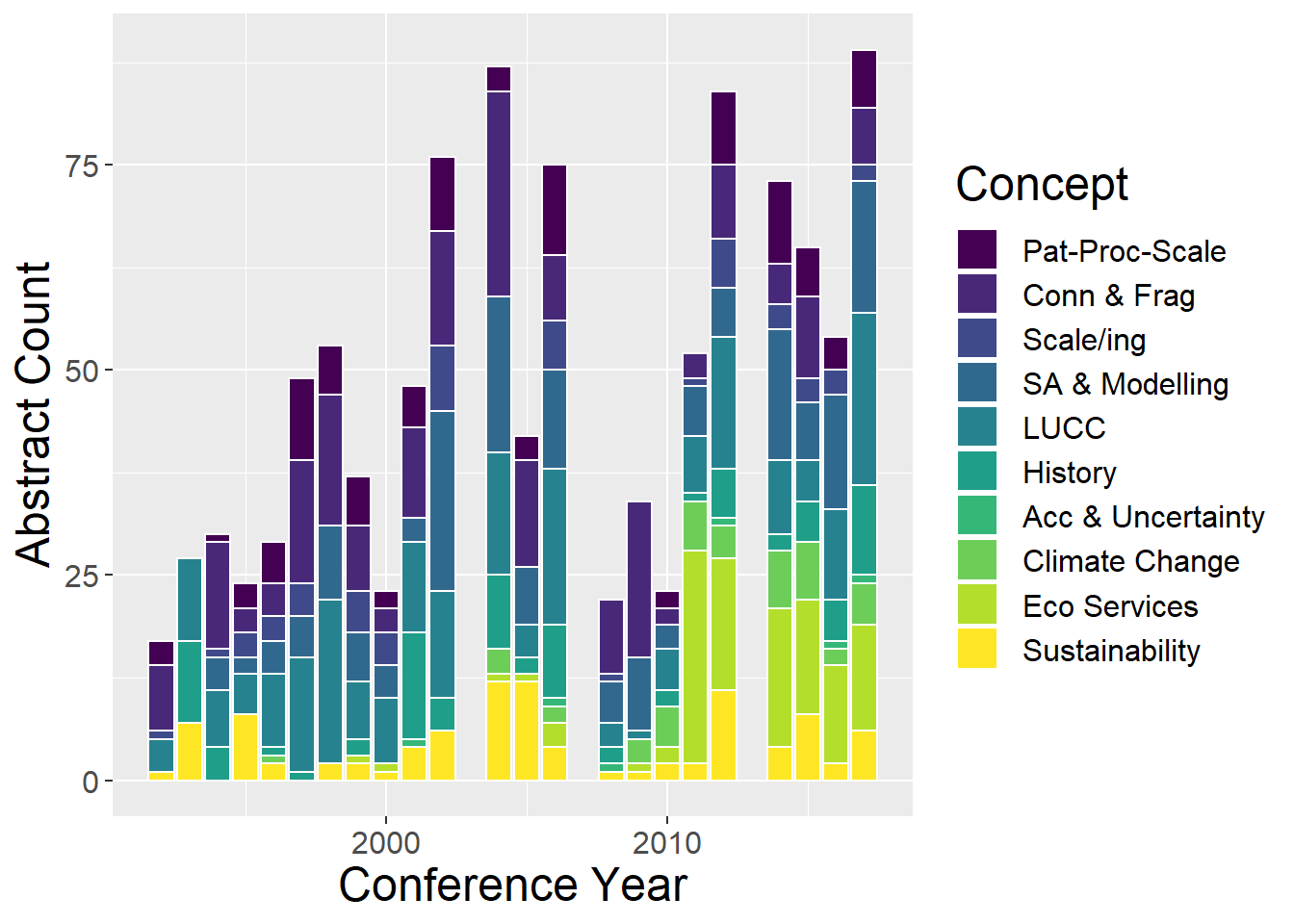

ggplot(conceptCounts, aes(x=`Conference Year`, y=prop, fill=factor(Type, level=factor_order))) +
  geom_bar(stat="identity", colour="white") +
  scale_fill_viridis(discrete = TRUE, labels = factor_labels) +
  labs(fill="Concept", y = "Proportion") +
  scale_x_continuous(breaks = seq(1992, 2017, by = 2))+
  theme(axis.text.x = element_text(angle = 40, hjust = 1))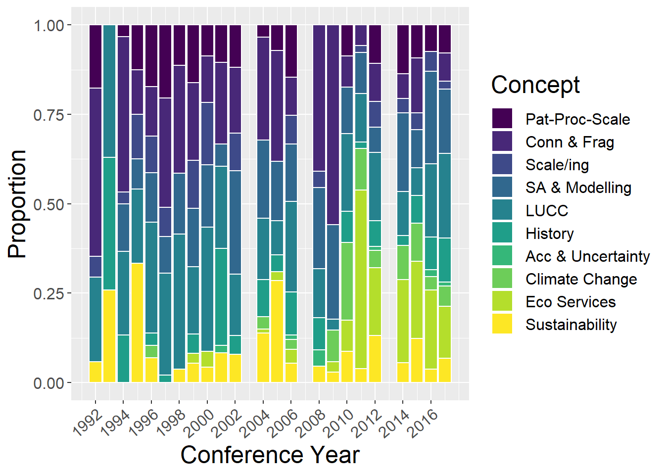 

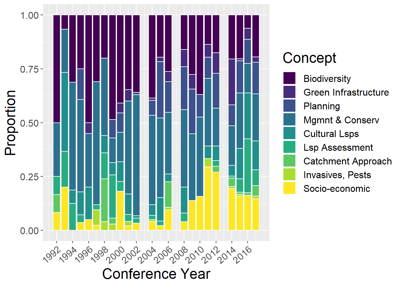
2.9 Other Concepts

General observations:

• Socio-economic studies have increased through time
• Biodiversity has decreased through time
• Landscape management and Biodiversity peak in early 2000s

othCCounts <- yrdata %>%
  select(`Conference Year`, `Green Infrastructure`,`Planning and Architecture`,`Management and Conservation`,`Cultural Landscapes`,`Socio-economic Dimensions`,Biodiversity,`Landscape Assessment`,`Catchment Based Approach`,`Invasives Pests Diseases`
) %>%
  mutate(yrsum = rowSums(.[2:10])) %>%
  gather(key = Type, value = count, -`Conference Year`, -yrsum) %>%
  mutate(prop = count / yrsum) 

yrdata %>%
  select(`Conference Year`, `Green Infrastructure`,`Planning and Architecture`,`Management and Conservation`,`Cultural Landscapes`,`Socio-economic Dimensions`,Biodiversity,`Landscape Assessment`,`Catchment Based Approach`,`Invasives Pests Diseases`
) %>%
  mutate(Total = rowSums(.[2:10])) %>%
  mutate_if(is.numeric, funs(prop = ./ Total)) %>%
  mutate_at(vars(ends_with("prop")), round, 3) %>% 
  select(-Total_prop) %>%
  kable() %>%
  kable_styling() %>%
  scroll_box(width = "100%", height= "400px")

Conference Year	Green Infrastructure	Planning and Architecture	Management and Conservation	Cultural Landscapes	Socio-economic Dimensions	Biodiversity	Landscape Assessment	Catchment Based Approach	Invasives Pests Diseases	Total	Conference Year_prop	Green Infrastructure_prop	Planning and Architecture_prop	Management and Conservation_prop	Cultural Landscapes_prop	Socio-economic Dimensions_prop	Biodiversity_prop	Landscape Assessment_prop	Catchment Based Approach_prop	Invasives Pests Diseases_prop
1992	0	0	3	0	1	6	1	1	0	12	166.000	0.000	0.000	0.250	0.000	0.083	0.500	0.083	0.083	0.000
1993	0	0	6	11	6	2	5	0	0	30	66.433	0.000	0.000	0.200	0.367	0.200	0.067	0.167	0.000	0.000
1994	0	0	8	1	0	5	2	0	0	16	124.625	0.000	0.000	0.500	0.062	0.000	0.312	0.125	0.000	0.000
1995	0	4	12	3	1	7	1	0	0	28	71.250	0.000	0.143	0.429	0.107	0.036	0.250	0.036	0.000	0.000
1996	1	0	5	3	1	10	0	0	0	20	99.800	0.050	0.000	0.250	0.150	0.050	0.500	0.000	0.000	0.000
1997	0	0	24	0	1	13	1	0	3	42	47.548	0.000	0.000	0.571	0.000	0.024	0.310	0.024	0.000	0.071
1998	0	0	9	2	0	5	3	5	1	25	79.920	0.000	0.000	0.360	0.080	0.000	0.200	0.120	0.200	0.040
1999	0	3	4	2	0	17	7	1	1	35	57.114	0.000	0.086	0.114	0.057	0.000	0.486	0.200	0.029	0.029
2000	1	2	3	2	4	9	1	0	0	22	90.909	0.045	0.091	0.136	0.091	0.182	0.409	0.045	0.000	0.000
2001	5	0	41	9	2	33	3	0	2	95	21.063	0.053	0.000	0.432	0.095	0.021	0.347	0.032	0.000	0.021
2002	0	1	50	1	3	32	2	0	0	89	22.494	0.000	0.011	0.562	0.011	0.034	0.360	0.022	0.000	0.000
2004	1	7	42	5	4	39	2	0	1	101	19.842	0.010	0.069	0.416	0.050	0.040	0.386	0.020	0.000	0.010
2005	1	12	17	5	1	9	1	0	0	46	43.587	0.022	0.261	0.370	0.109	0.022	0.196	0.022	0.000	0.000
2006	4	12	24	3	8	22	0	10	1	84	23.881	0.048	0.143	0.286	0.036	0.095	0.262	0.000	0.119	0.012
2008	2	5	9	3	1	4	1	0	0	25	80.320	0.080	0.200	0.360	0.120	0.040	0.160	0.040	0.000	0.000
2009	2	6	9	0	4	8	0	0	0	29	69.276	0.069	0.207	0.310	0.000	0.138	0.276	0.000	0.000	0.000
2010	0	2	7	0	3	7	0	0	0	19	105.789	0.000	0.105	0.368	0.000	0.158	0.368	0.000	0.000	0.000
2011	3	5	16	3	15	7	0	0	2	51	39.431	0.059	0.098	0.314	0.059	0.294	0.137	0.000	0.000	0.039
2012	7	12	13	5	20	13	2	2	0	74	27.189	0.095	0.162	0.176	0.068	0.270	0.176	0.027	0.027	0.000
2014	22	10	19	5	20	21	1	4	1	103	19.553	0.214	0.097	0.184	0.049	0.194	0.204	0.010	0.039	0.010
2015	1	17	29	16	18	23	7	1	1	113	17.832	0.009	0.150	0.257	0.142	0.159	0.204	0.062	0.009	0.009
2016	4	9	11	17	13	5	20	1	0	80	25.200	0.050	0.112	0.138	0.212	0.162	0.062	0.250	0.012	0.000
2017	2	12	18	11	12	16	6	4	1	82	24.598	0.024	0.146	0.220	0.134	0.146	0.195	0.073	0.049	0.012

factor_order <- c('Biodiversity','Green Infrastructure','Planning and Architecture','Management and Conservation','Cultural Landscapes','Landscape Assessment','Catchment Based Approach','Invasives Pests Diseases','Socio-economic Dimensions')
factor_labels <- c('Biodiversity','Green Infrastructure','Planning','Mgmnt & Conserv','Cultural Lsps','Lsp Assessment','Catchment Approach','Invasives, Pests','Socio-economic')

ggplot(othCCounts, aes(x=`Conference Year`, y=count, fill=factor(Type, level=factor_order))) +
  geom_bar(stat="identity", colour="white") +
  scale_fill_viridis(discrete = TRUE, labels = factor_labels) +
  labs(fill="Concept", y = "Abstract Count")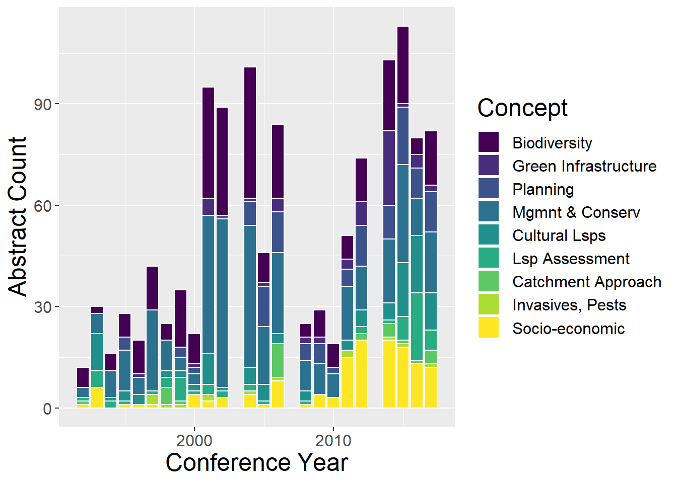

ggplot(othCCounts, aes(x=`Conference Year`, y=prop, fill=factor(Type, level=factor_order))) +
  geom_bar(stat="identity", colour="white") +
  scale_fill_viridis(discrete = TRUE, labels = factor_labels) +
  labs(fill="Concept", y = "Proportion") +
  scale_x_continuous(breaks = seq(1992, 2017, by = 2))+
  theme(axis.text.x = element_text(angle = 40, hjust = 1))