Chapter 5 Analysis by Organism

Bar charts and tables to examine how contributions to conferences vary by organism

5.1 Total Conference Contributions

#spec(cpdata)

sppdata <- cpdata %>%
  select_if(is.numeric) %>%
  gather(key = SppType, value = count, Mammals:Fish) %>%
  filter(count > 0) %>%
  group_by(`SppType`) %>%
  summarise_all(sum, na.rm=T) 

General observations:

• Amphibians, Fish, Reptiles are little studied

sppdata %>%
  select(SppType, count) %>%
  mutate(prop = count/sum(count)) %>%
  mutate(prop = round(prop,3)) %>% 
  kable() %>%
  kable_styling() %>%
  scroll_box(width = "100%")

SppType	count	prop
Amphibians	11	0.022
Birds	128	0.256
Fish	11	0.022
Humans	79	0.158
Inverts	104	0.208
Mammals	43	0.086
Plants	119	0.238
Reptiles	5	0.010

ggplot(sppdata, aes(x=SppType, y=count)) + 
  geom_bar(stat="identity") + 
  geom_text(aes(x=SppType, y=max(count), label = paste0(round(100*count / sum(count),1), "%"), vjust=-0.25)) +
  labs(y = "Abstract Count", x="Organism")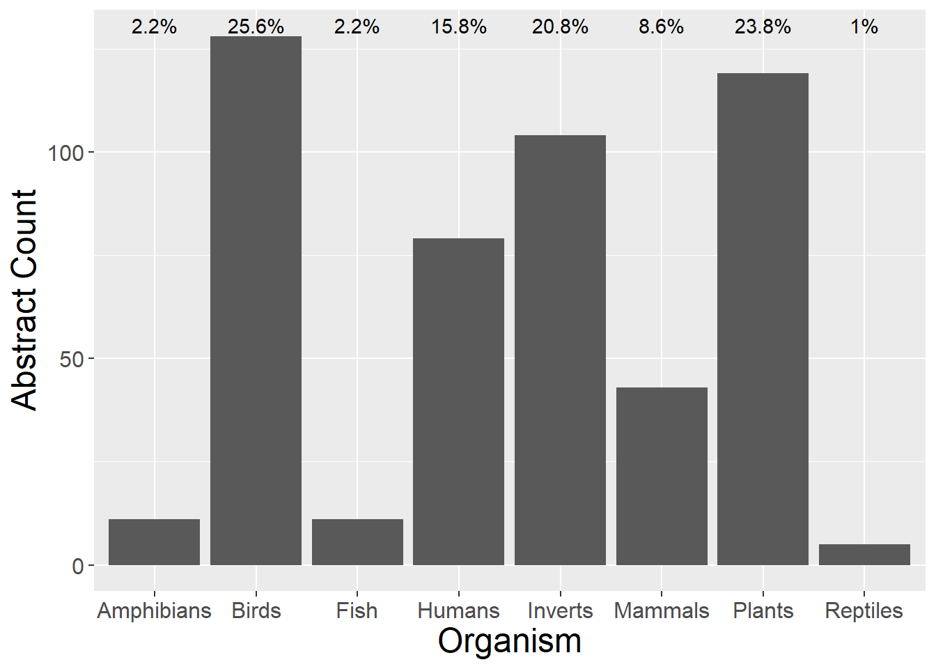

5.2 Author Affiliation

General observations:

• Businesses and private individuals study humans (proportional)
• By absolute numbers NGOs dominate study of birds

authorCounts <- sppdata %>%
  select(SppType,Academic, Government,NGO,Business,Private) %>%
  mutate(sum = rowSums(.[2:6])) %>%   #calculate total for subsquent calcultation of proportion
  gather(key = Type, value = count, -SppType, -sum) %>%
  mutate(prop = count / sum)  #calculate proportion

ggplot(authorCounts, aes(x=SppType, y=count, fill=Type)) + geom_bar(stat="identity", colour="white") +
  scale_fill_viridis(discrete = TRUE) +
  theme(axis.text.x = element_text(angle = 30, hjust = 1)) +
  labs(fill="Affiliation", y = "Abstract Count", x="Organism")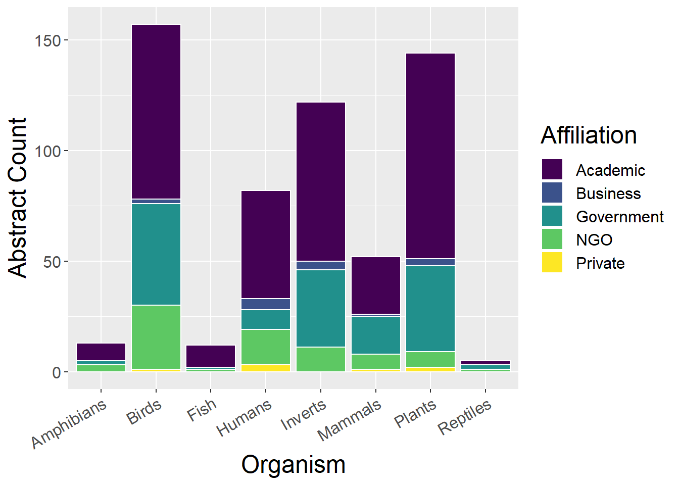

ggplot(authorCounts, aes(x=SppType, y=prop, fill=Type)) + geom_bar(stat="identity", colour="white") +
  scale_fill_viridis(discrete = TRUE) +
  theme(axis.text.x = element_text(angle = 30, hjust = 1)) +
  labs(fill="Affiliation", y = "Proportion", x="Organism")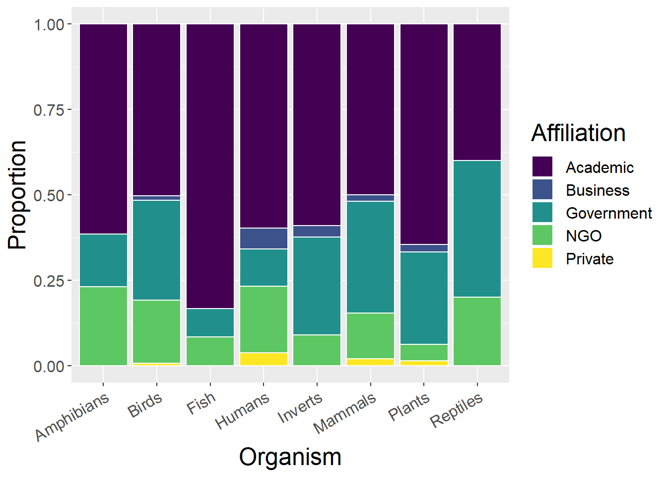

5.3 Landscape Type

5.3.1 Using all landscape types

General observations:

• Human studies are most evenly distributed across landscape types
• Unsurprisingly, fish are studies in riverscapes and seascapes
• Birds, plants and inverts studies dominated by Lowland rural studies

lspCounts <- sppdata %>%
  select(SppType,`Upland rural`, `Lowland rural`, Urban,    Riverscape, Seascape, `Undefined LspType`,Other) %>%
  mutate(sum = rowSums(.[2:8])) %>%   #calculate total for subsquent calcultation of proportion
  gather(key = Type, value = count, -SppType, -sum) %>%
  mutate(prop = count / sum)  #calculate proportion

ggplot(lspCounts, aes(x=SppType, y=count, fill=Type)) + geom_bar(stat="identity", colour="white") +
  scale_fill_viridis(discrete = TRUE) +
  theme(axis.text.x = element_text(angle = 30, hjust = 1)) +
  labs(fill="Landscape Type", y = "Abstract Count", x="Organism")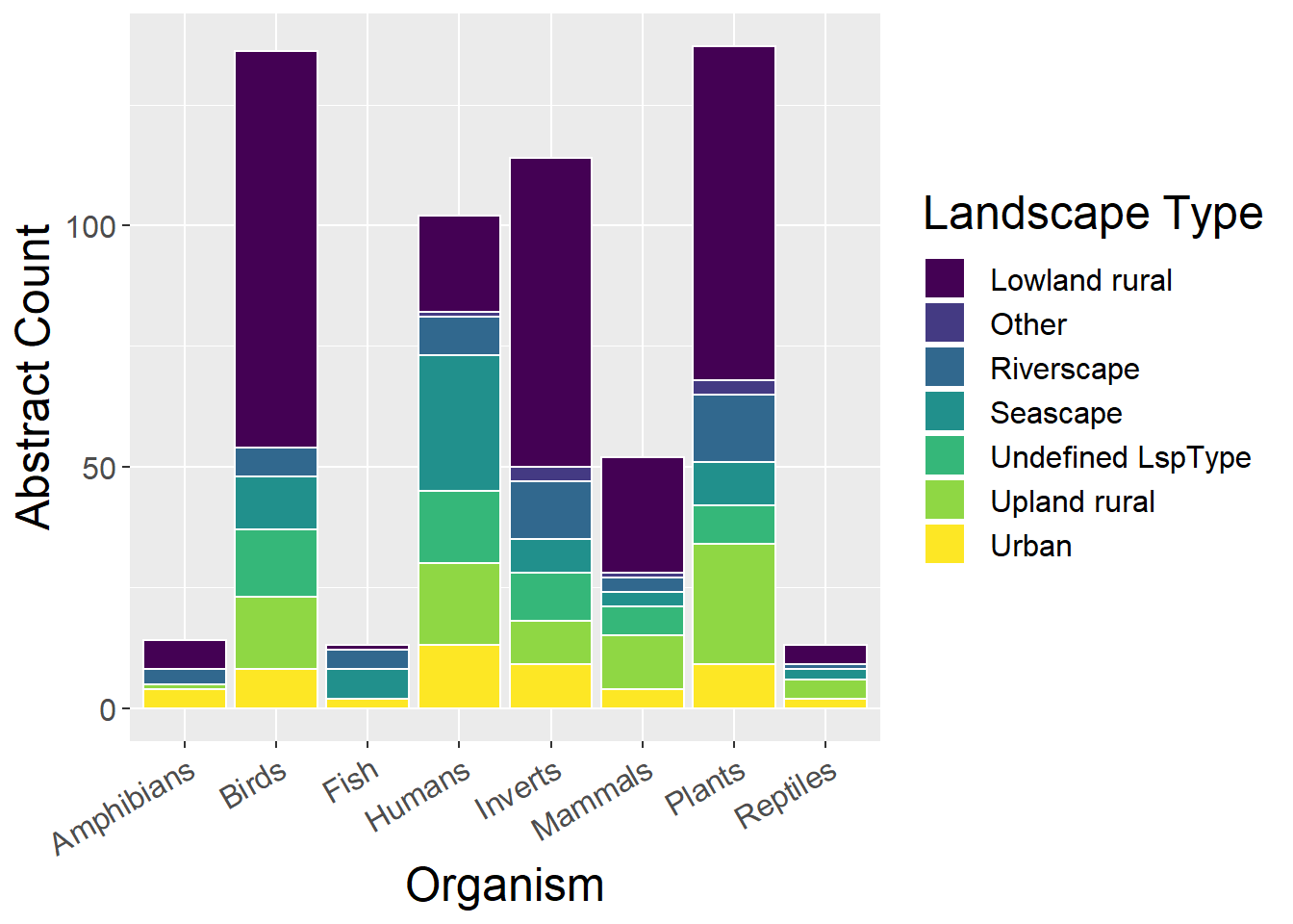

ggplot(lspCounts, aes(x=SppType, y=prop, fill=Type)) + geom_bar(stat="identity", colour="white") +
  scale_fill_viridis(discrete = TRUE) +
  theme(axis.text.x = element_text(angle = 30, hjust = 1)) +
  labs(fill="Landscape Type", y = "Proportion", x="Organism")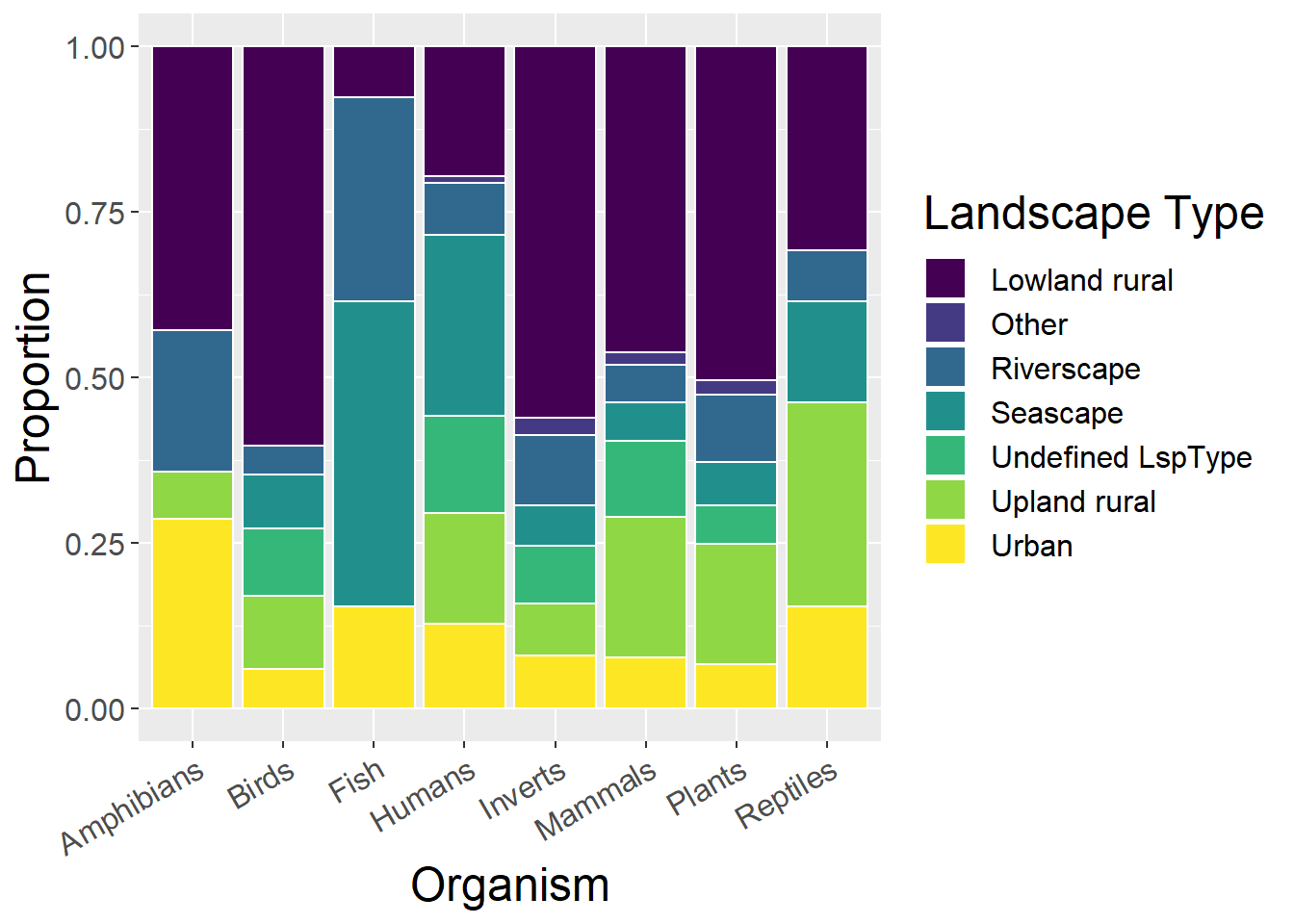

5.3.2 Without ‘Undefined LspType’ and ‘Other’ landscape types

General observations:

• Birds, Plants and Mammals studies predominantly in Lowland Rural lsps
• Plants studies are greatest contribution (in total number) to Upland Rural lsps

lspCounts <- sppdata %>%
  select(SppType,`Upland rural`, `Lowland rural`, Urban,    Riverscape, Seascape) %>%
  mutate(sum = rowSums(.[2:6])) %>%   #calculate total for subsquent calcultation of proportion
  gather(key = Type, value = count, -SppType, -sum) %>%
  mutate(prop = count / sum)  #calculate proportion

ggplot(lspCounts, aes(x=SppType, y=count, fill=Type)) + geom_bar(stat="identity", colour="white") +
  scale_fill_viridis(discrete = TRUE) +
  theme(axis.text.x = element_text(angle = 30, hjust = 1)) +
  labs(fill="Landscape Type", y = "Abstract Count", x="Organism")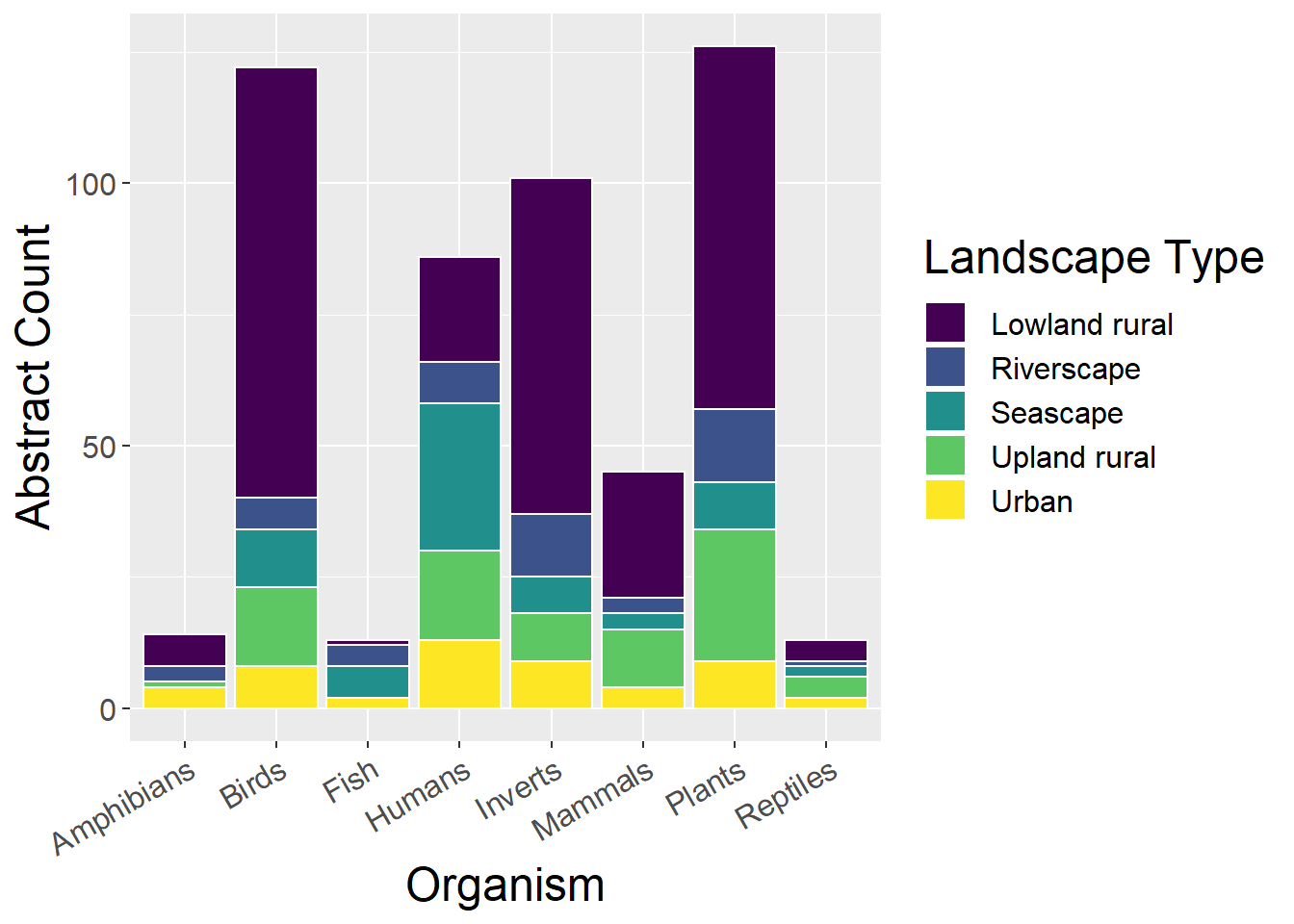

ggplot(lspCounts, aes(x=SppType, y=prop, fill=Type)) + geom_bar(stat="identity", colour="white") +
  scale_fill_viridis(discrete = TRUE) +
  theme(axis.text.x = element_text(angle = 30, hjust = 1)) +
  labs(fill="Landscape Type", y = "Proportion", x="Organism")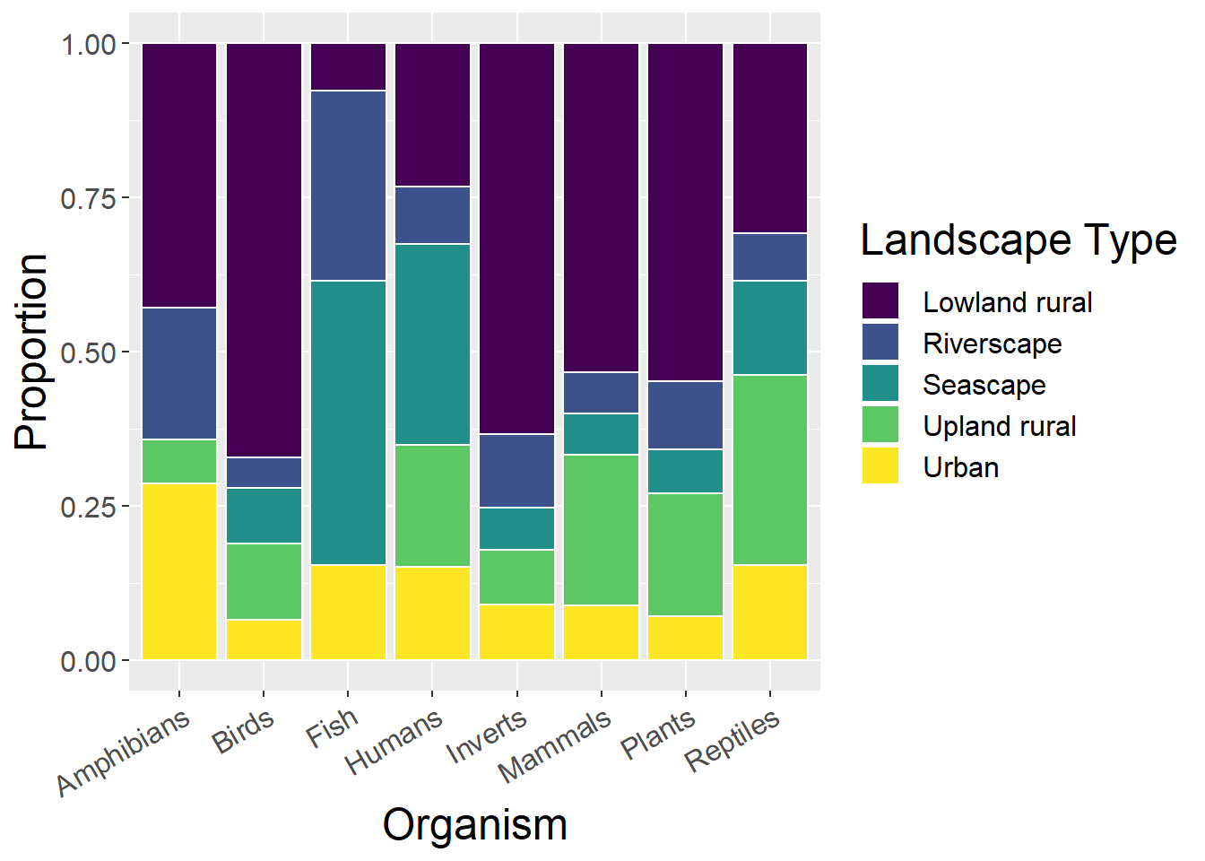

5.4 Methods

General observations:

• Humans dominated by qualitative studies, with few empirical (i.e. few interviews, questionnaires?)
• Possibly surprisingly, plants do not have many RS studies

methodsCounts <- sppdata %>%
  select(SppType, Empirical, Theoretical, Qualitative, Quantitative, GIS, `Remote sensing`) %>%
  mutate(sum = rowSums(.[2:7])) %>%
  gather(key = Type, value = count, -SppType, -sum) %>%
  mutate(prop = count / sum) 

ggplot(methodsCounts, aes(x=SppType, y=count, fill=Type)) + geom_bar(stat="identity", colour="white") +
  scale_fill_viridis(discrete = TRUE) +
  theme(axis.text.x = element_text(angle = 30, hjust = 1)) +
  labs(fill="Method", y = "Abstract Count", x="Organism")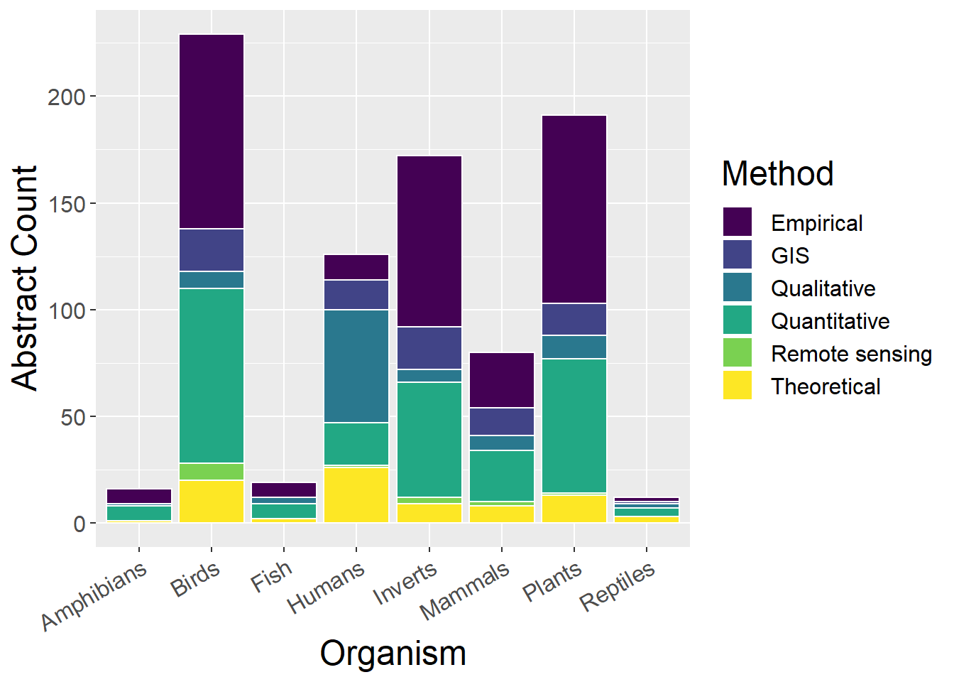

ggplot(methodsCounts, aes(x=SppType, y=prop, fill=Type)) + geom_bar(stat="identity", colour="white") +
  scale_fill_viridis(discrete = TRUE) +
  theme(axis.text.x = element_text(angle = 30, hjust = 1)) +
  labs(fill="Method", y = "Proportion", x="Organism")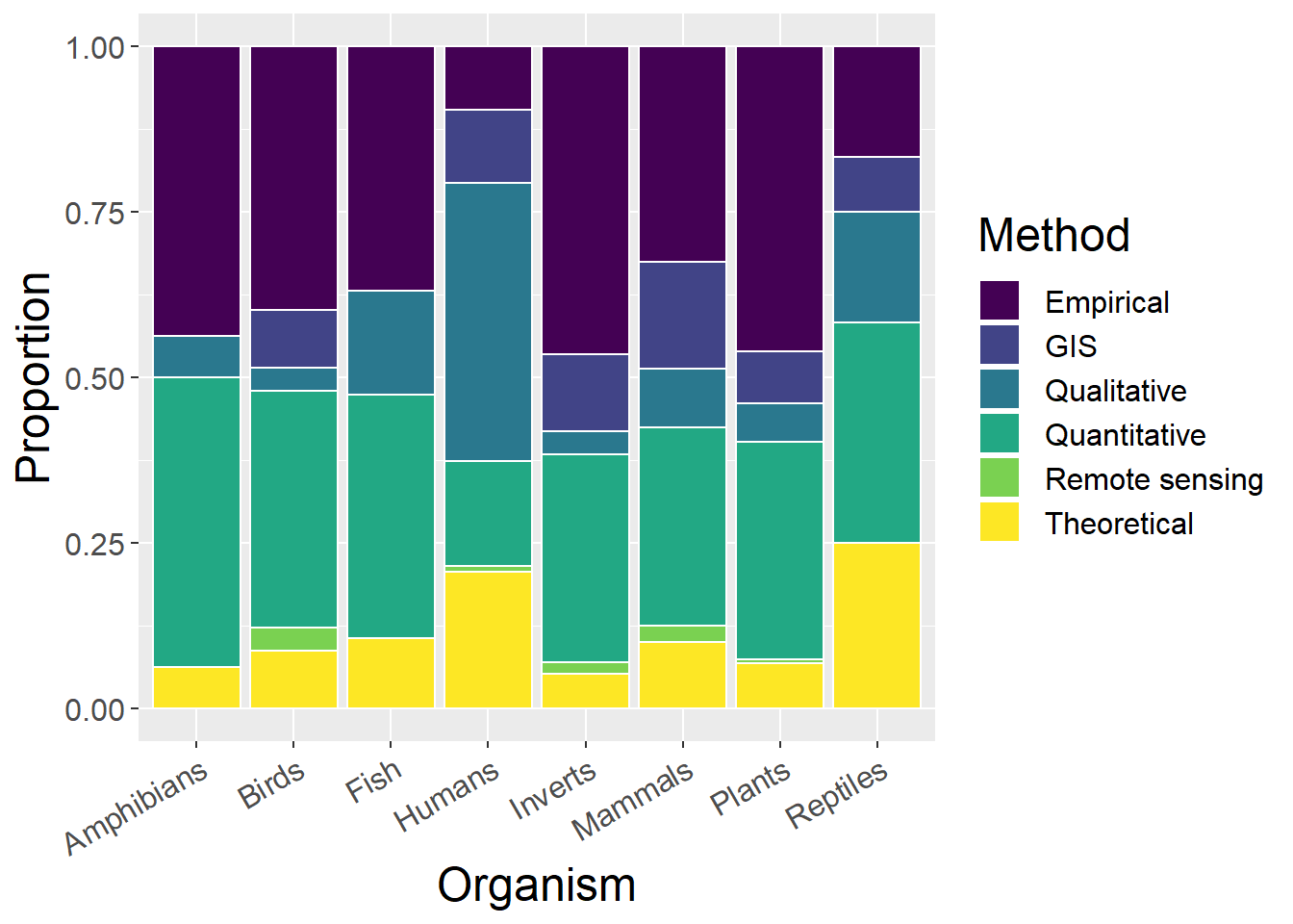

5.5 Spatial Extent

General observations:

• Inverts dominated by mini studies
• Fish have relatively high proportion of Global studies
• Other species have reasonably evenly distributed proportions of scales

spatialCounts <- sppdata %>%
  select(SppType, Micro, Mini, Local, Regional, National, Continental, Global,`Undefined Extent`) %>%
  mutate(sum = rowSums(.[2:9])) %>%
  gather(key = Type, value = count, -SppType, -sum) %>%
  mutate(prop = count / sum) 

factor_order <- c('Micro', 'Mini', 'Local', 'Regional', 'National', 'Continental', 'Global','Undefined Extent')
factor_labels <- c('Micro', 'Mini', 'Local', 'Regional', 'National', 'Continental', 'Global','Undefined')

ggplot(spatialCounts, aes(x=SppType, y=count, fill=factor(Type, level=factor_order))) + geom_bar(stat="identity", colour="white")  +
  scale_fill_viridis(discrete = TRUE) +
  theme(axis.text.x = element_text(angle = 30, hjust = 1)) +
  labs(fill="Extent", y = "Abstract Count", x="Organism")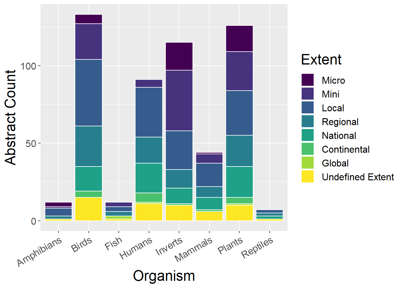

ggplot(spatialCounts, aes(x=SppType, y=prop, fill=factor(Type, level=factor_order))) + geom_bar(stat="identity", colour="white")  +
  scale_fill_viridis(discrete = TRUE) +
  theme(axis.text.x = element_text(angle = 30, hjust = 1)) +
  labs(fill="Extent", y = "Proportion", x="Organism")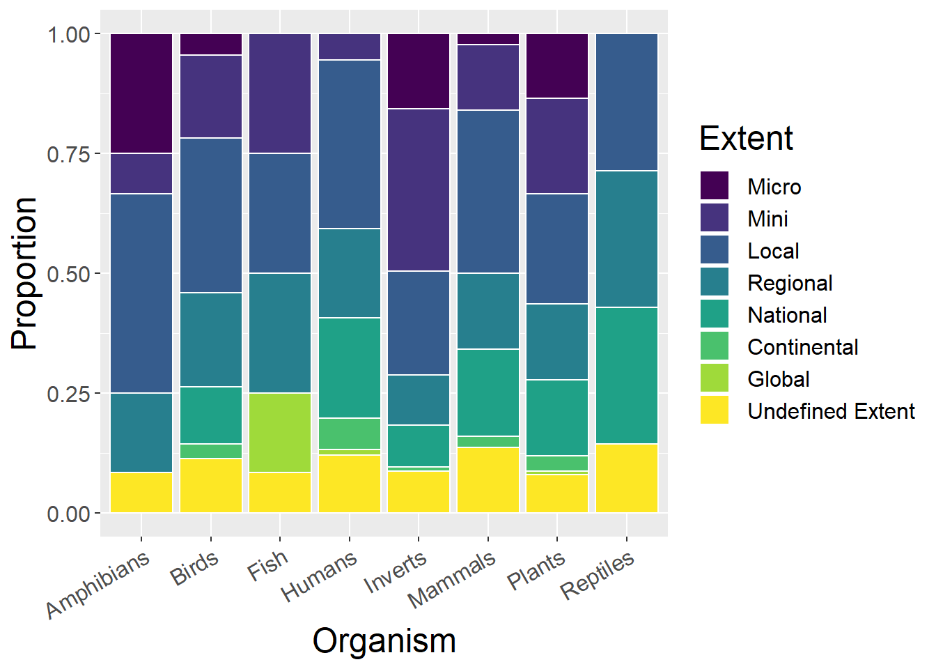

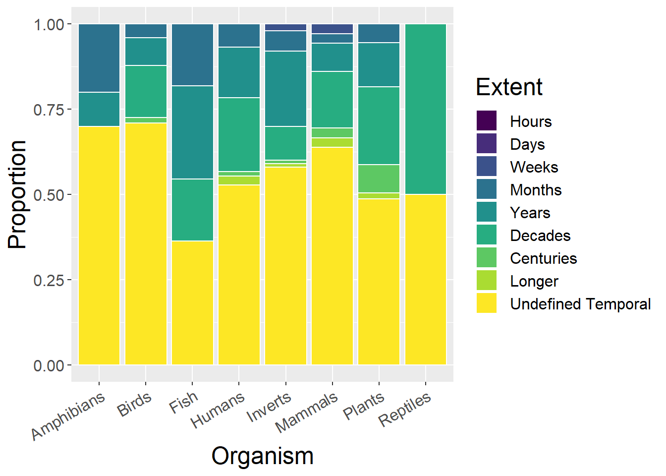
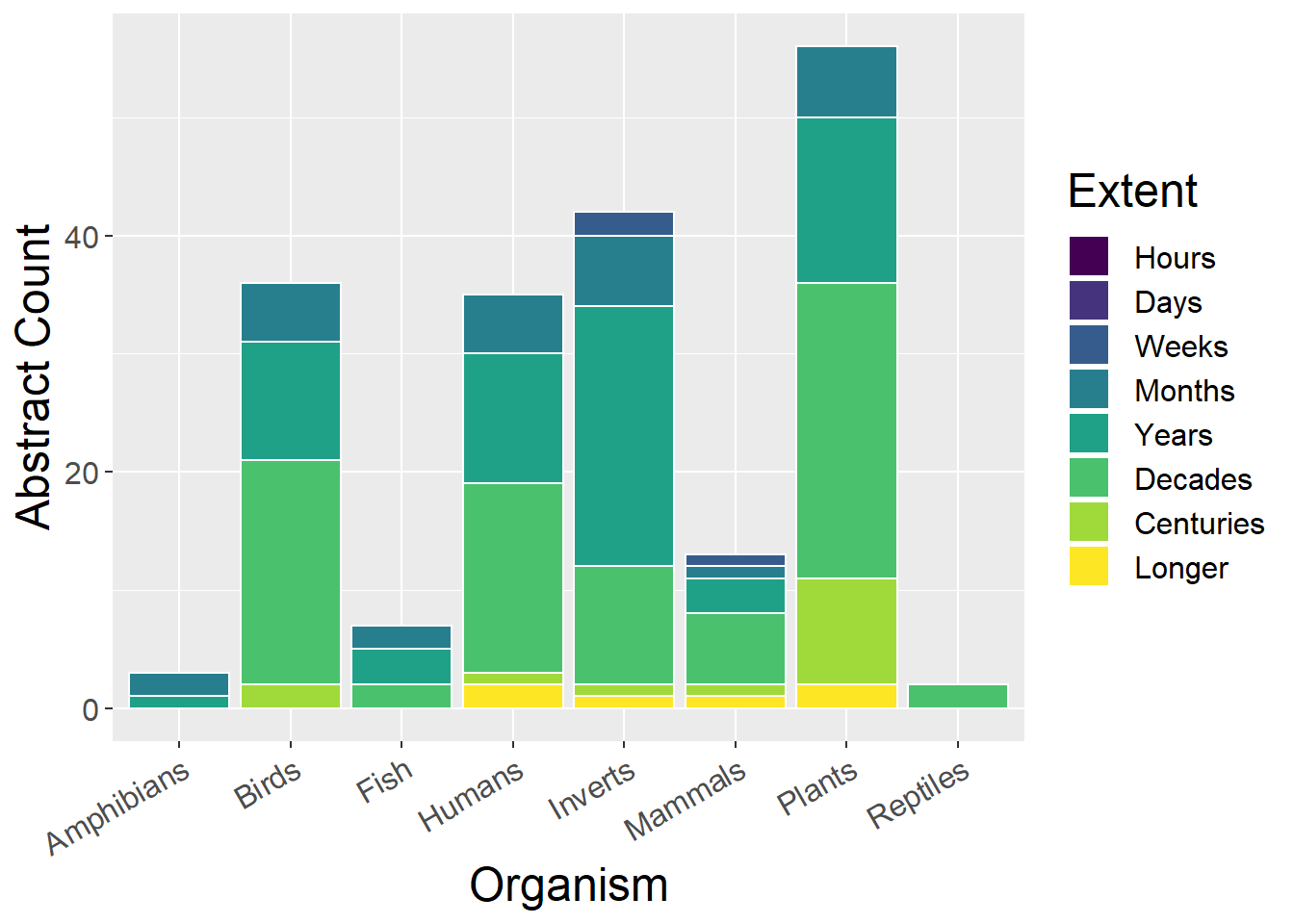
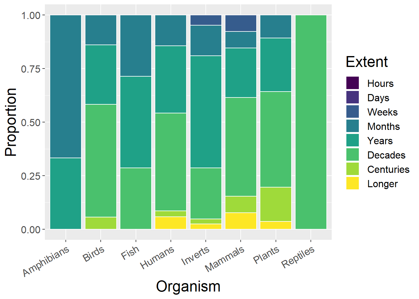
5.6 Temporal Extent

5.6.1 With undefined

General observations:

• Difficult to see much; examine without ‘undefined’

5.6.2 Without Undefined

General observations:

• Inverts dominated by annual (Yearly) studies, plus shorter studies
• Plants have greatest proportions of longer studies (Decadal and Centuries) - makes sense given rates of change?

5.7 Concepts

General observations:

• Humans have a relatively large proportion of Ecosystem Services studies (not surprising?)
• Plants have largest number of LUCC studies

conceptCounts <- sppdata %>%
  select(SppType, `PPS of landscapes`,
`Connectivity and fragmentation`, `Scale and scaling`,`Spatial analysis and modeling`,LUCC,`History and legacy`,`Climate change interactions`,`Ecosystem services`,`Landscape sustainability`,`Accuracy and uncertainty`
) %>%
  mutate(sum = rowSums(.[2:11])) %>%
  gather(key = Type, value = count, -SppType, -sum) %>%
  mutate(prop = count / sum) 

ggplot(conceptCounts, aes(x=SppType, y=count, fill=Type)) + 
  geom_bar(stat="identity", colour="white")  +
  scale_fill_viridis(discrete = TRUE) +
  theme(axis.text.x = element_text(angle = 30, hjust = 1)) +
  labs(fill="Concept", y = "Abstract Count", x="Organism")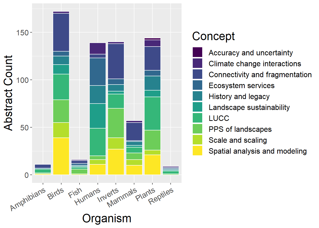

ggplot(conceptCounts, aes(x=SppType, y=prop, fill=Type)) + 
  geom_bar(stat="identity", colour="white")  +
  scale_fill_viridis(discrete = TRUE) +
  theme(axis.text.x = element_text(angle = 30, hjust = 1)) +
  labs(fill="Concept", y = "Proportion", x="Organism")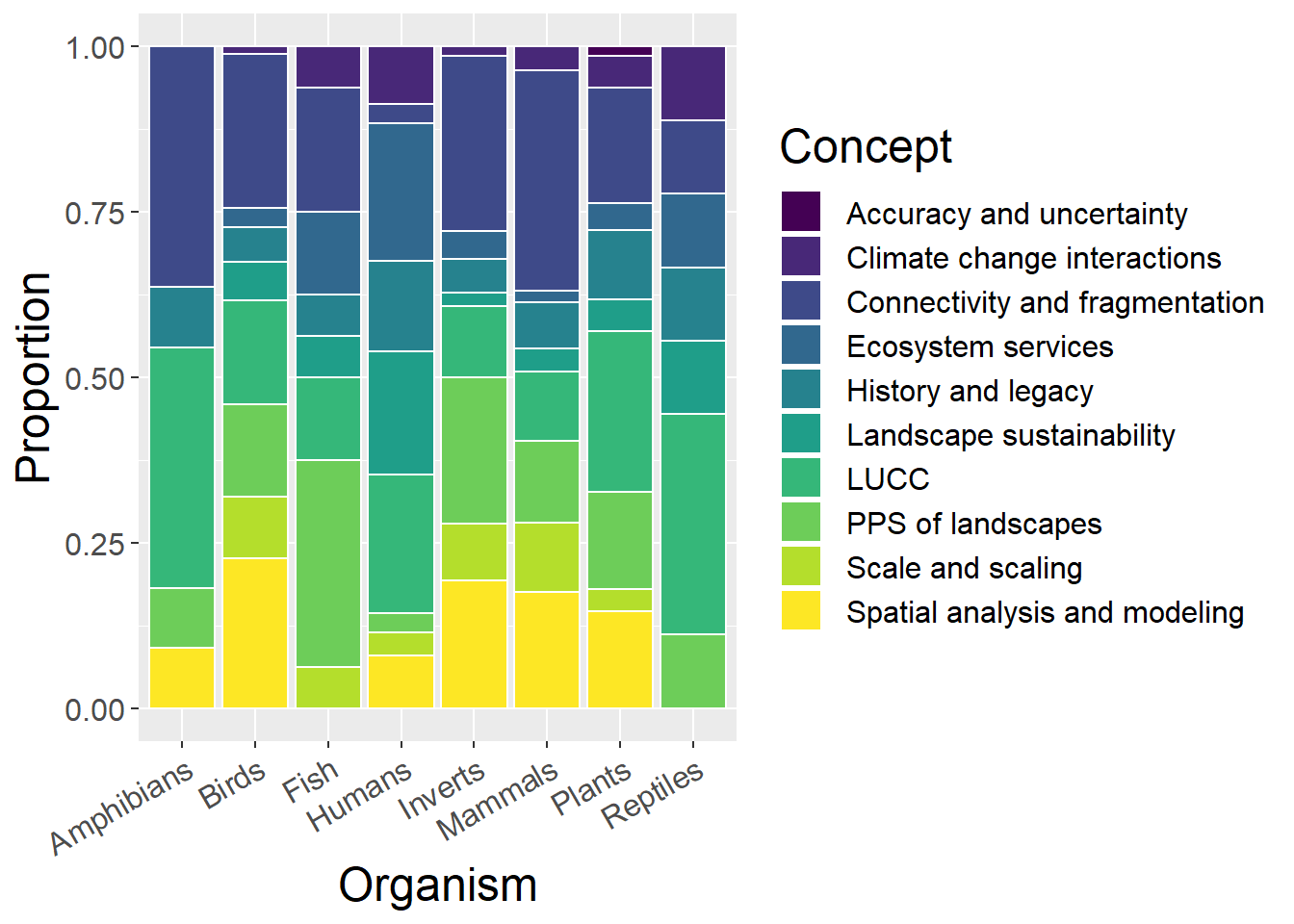

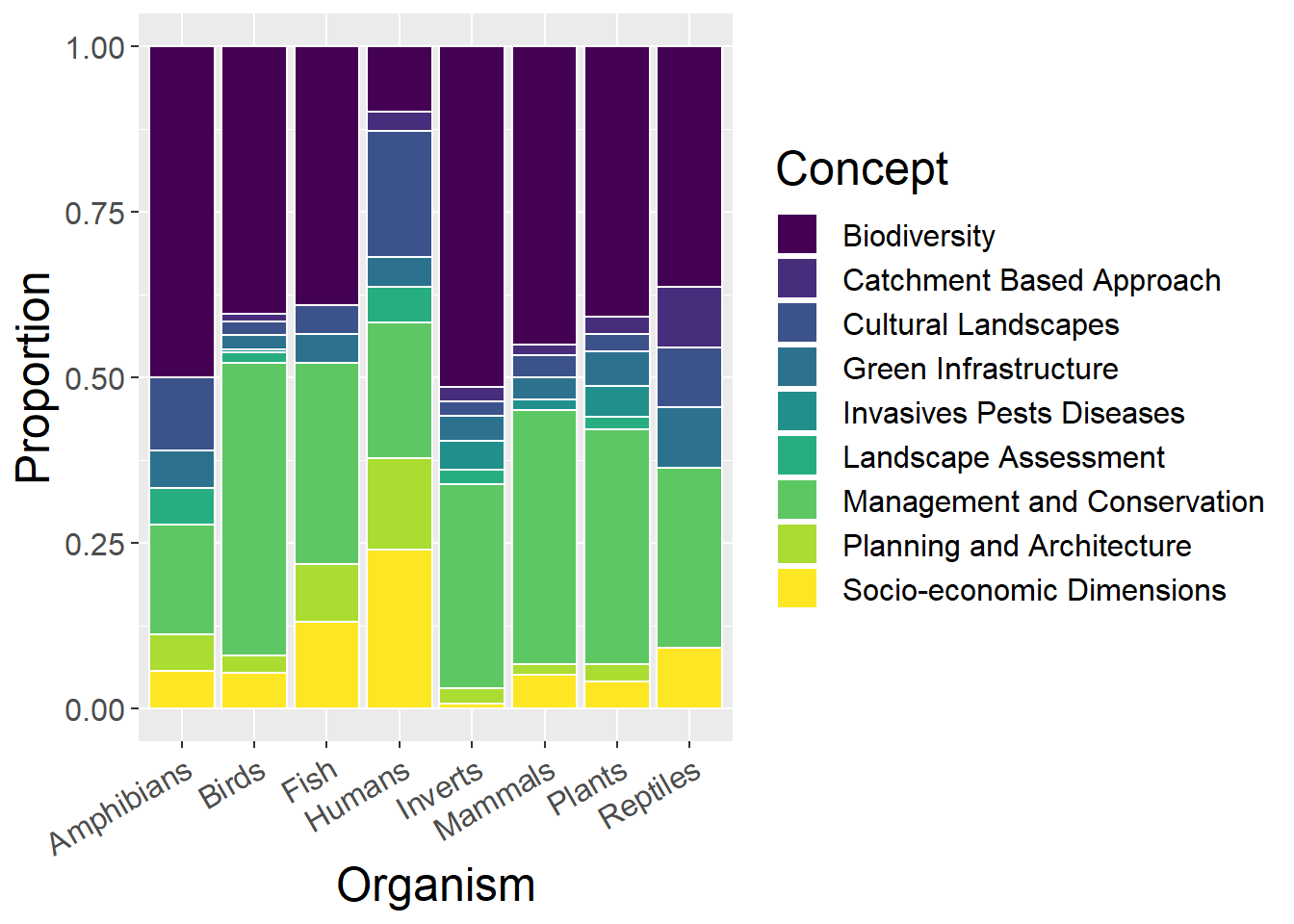
5.8 Other Concepts

General observations:

• Humans have largest proportion of Cultural Landscapes, Socio-Economic and Planning studies (unsurprising?)
• Birds, Inverts and Mammals dominates by biodiveristy and Management and Conservation studies

othCCounts <- sppdata %>%
  select(SppType, `Green Infrastructure`,`Planning and Architecture`,`Management and Conservation`,`Cultural Landscapes`,`Socio-economic Dimensions`,Biodiversity,`Landscape Assessment`,`Catchment Based Approach`,`Invasives Pests Diseases`
) %>%
  mutate(sum = rowSums(.[2:10])) %>%
  gather(key = Type, value = count, -SppType, -sum) %>%
  mutate(prop = count / sum) 

ggplot(othCCounts, aes(x=SppType, y=count, fill=Type)) + geom_bar(stat="identity", colour="white") +
  scale_fill_viridis(discrete = TRUE) +
  theme(axis.text.x = element_text(angle = 30, hjust = 1)) +
  labs(fill="Concept", y = "Abstract Count", x="Organism")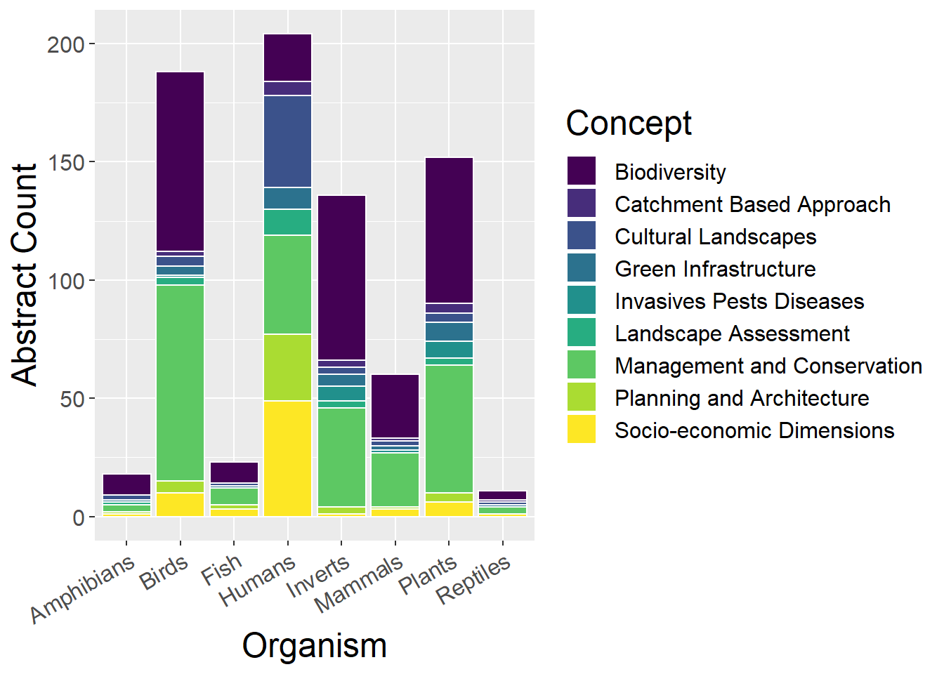

ggplot(othCCounts, aes(x=SppType, y=prop, fill=Type)) + geom_bar(stat="identity", colour="white") +
  scale_fill_viridis(discrete = TRUE) +
  theme(axis.text.x = element_text(angle = 30, hjust = 1)) +
  labs(fill="Concept", y = "Proportion", x="Organism")