Chapter 10 Analysis by Other Concepts | 25 years of ialeUK conferences: An analysis

10.1 Total Conference Contributions

General observations:

Invasive pests have smallest number of studies (and therefore treat qualitative differences in proportions below with caution)
Management & Conservation and Biodiversity studies componse the majority of studies (56%)

othdata %>%
  select(OtherC, count) %>%
  mutate(prop = count/sum(count)) %>%
  mutate(prop = round(prop,3)) %>% 
  kable() %>%
  kable_styling() %>%
  scroll_box(width = "100%")

OtherC	count	prop
Biodiversity	313	0.256
Catchment Based Approach	29	0.024
Cultural Landscapes	107	0.088
Green Infrastructure	56	0.046
Invasives Pests Diseases	14	0.011
Landscape Assessment	66	0.054
Management and Conservation	379	0.310
Planning and Architecture	119	0.097
Socio-economic Dimensions	138	0.113

ggplot(othdata, aes(x=OtherC, y=count)) + 
  geom_bar(stat="identity") + 
  geom_text(aes(x=OtherC, y=max(count), label = paste0(round(100*count / sum(count),1), "%"), vjust=-0.25)) + 
  theme(axis.text.x = element_text(angle = 25, hjust = 1))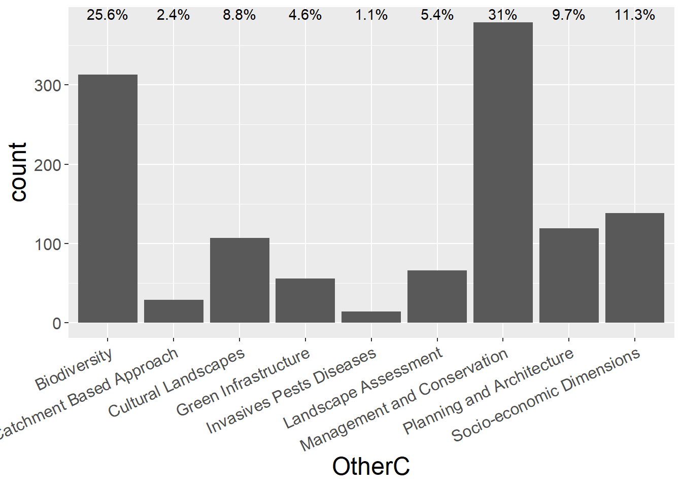

10.2 Author Affiliation

General observations:

No obvious differences (other than invasive pests which has small numbers)

authCounts <- othdata %>%
  select(OtherC,Academic, Government,NGO,Business,Private) %>%
  mutate(sum = rowSums(.[2:6])) %>%   #calculate total for subsquent calcultation of proportion
  gather(key = Type, value = count, -OtherC, -sum) %>%
  mutate(prop = count / sum)  #calculate proportion

othdata %>%
  select(OtherC,Academic, Government,NGO,Business,Private) %>%
  mutate(Total = rowSums(.[2:6])) %>%   #calculate total
  mutate_if(is.numeric, funs(prop = ./ Total)) %>%
  mutate_at(vars(ends_with("prop")), round, 3) %>% 
  select(-Total_prop) %>%
  kable() %>%
  kable_styling() %>%
  scroll_box(width = "100%")

OtherC	Academic	Government	NGO	Business	Private	Total	Academic_prop	Government_prop	NGO_prop	Business_prop	Private_prop
Biodiversity	189	90	54	23	5	361	0.524	0.249	0.150	0.064	0.014
Catchment Based Approach	19	7	6	3	0	35	0.543	0.200	0.171	0.086	0.000
Cultural Landscapes	71	21	9	8	4	113	0.628	0.186	0.080	0.071	0.035
Green Infrastructure	34	12	6	5	2	59	0.576	0.203	0.102	0.085	0.034
Invasives Pests Diseases	7	7	0	1	0	15	0.467	0.467	0.000	0.067	0.000
Landscape Assessment	37	22	1	4	4	68	0.544	0.324	0.015	0.059	0.059
Management and Conservation	218	118	77	24	11	448	0.487	0.263	0.172	0.054	0.025
Planning and Architecture	64	27	18	10	6	125	0.512	0.216	0.144	0.080	0.048
Socio-economic Dimensions	90	24	19	8	3	144	0.625	0.167	0.132	0.056	0.021

ggplot(authCounts, aes(x=OtherC, y=count, fill=Type)) + 
  geom_bar(stat="identity", colour="white") + 
  theme(axis.text.x = element_text(angle = 45, hjust = 1)) +
  scale_fill_viridis(discrete = TRUE) +
  labs(fill="Affiliation", y = "Abstract Count", x="Concept")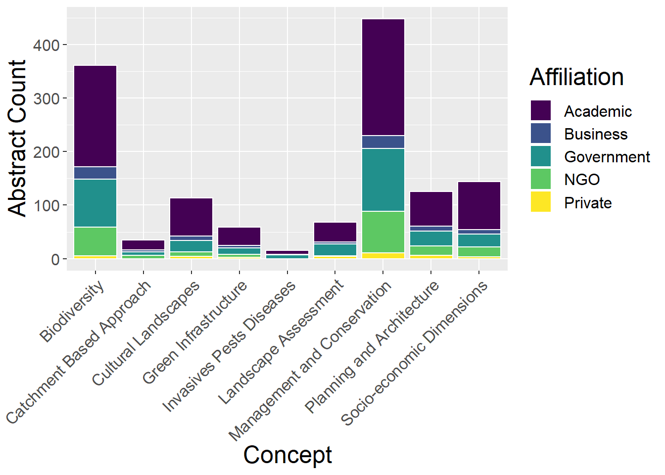

ggplot(authCounts, aes(x=OtherC, y=prop, fill=Type)) + 
  geom_bar(stat="identity", colour="white") + 
  theme(axis.text.x = element_text(angle = 45, hjust = 1)) +
  scale_fill_viridis(discrete = TRUE) +
  labs(fill="Affiliation", y = "Proportion", x="Concept")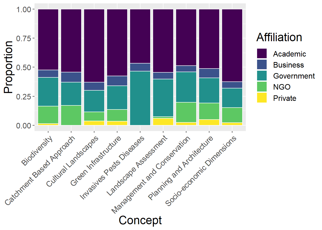

10.3 Landscape Type

10.3.1 Using all landscape types

General observations:

Green infrastructure has by far greatest proportion of Urban landscape studies (makes sense)
Catchment approaches have greatest proportion of Riverscapes (makes sense)

lspCounts <- othdata %>%
  select(OtherC,`Upland rural`, `Lowland rural`, Urban, Riverscape, Seascape, `Undefined LspType`,Other) %>%
  mutate(sum = rowSums(.[2:8])) %>%   #calculate total for subsquent calcultation of proportion
  gather(key = Type, value = count, -OtherC, -sum) %>%
  mutate(prop = count / sum)  #calculate proportion

othdata %>%
  select(OtherC,`Upland rural`, `Lowland rural`, Urban, Riverscape, Seascape, `Undefined LspType`,Other) %>%
  mutate(Total = rowSums(.[2:8])) %>%   #calculate total
  mutate_if(is.numeric, funs(prop = ./ Total)) %>%
  mutate_at(vars(ends_with("prop")), round, 3) %>% 
  select(-Total_prop) %>%
  kable() %>%
  kable_styling() %>%
  scroll_box(width = "100%")

OtherC	Upland rural	Lowland rural	Urban	Riverscape	Seascape	Undefined LspType	Other	Total	Upland rural_prop	Lowland rural_prop	Urban_prop	Riverscape_prop	Seascape_prop	Undefined LspType_prop	Other_prop
Biodiversity	33	156	45	33	32	39	12	350	0.094	0.446	0.129	0.094	0.091	0.111	0.034
Catchment Based Approach	5	6	6	19	2	3	0	41	0.122	0.146	0.146	0.463	0.049	0.073	0.000
Cultural Landscapes	20	38	9	6	22	25	5	125	0.160	0.304	0.072	0.048	0.176	0.200	0.040
Green Infrastructure	4	11	36	5	5	6	1	68	0.059	0.162	0.529	0.074	0.074	0.088	0.015
Invasives Pests Diseases	1	8	1	1	1	1	0	13	0.077	0.615	0.077	0.077	0.077	0.077	0.000
Landscape Assessment	17	26	7	4	14	19	6	93	0.183	0.280	0.075	0.043	0.151	0.204	0.065
Management and Conservation	56	177	34	45	43	54	13	422	0.133	0.419	0.081	0.107	0.102	0.128	0.031
Planning and Architecture	9	28	24	13	27	26	1	128	0.070	0.219	0.188	0.102	0.211	0.203	0.008
Socio-economic Dimensions	23	40	31	21	28	30	1	174	0.132	0.230	0.178	0.121	0.161	0.172	0.006

ggplot(lspCounts, aes(x=OtherC, y=count, fill=Type)) + 
  geom_bar(stat="identity", colour="white") + 
  theme(axis.text.x = element_text(angle = 45, hjust = 1)) +
  scale_fill_viridis(discrete = TRUE) +
  labs(fill="Landscape", y = "Abstract Count", x="Concept")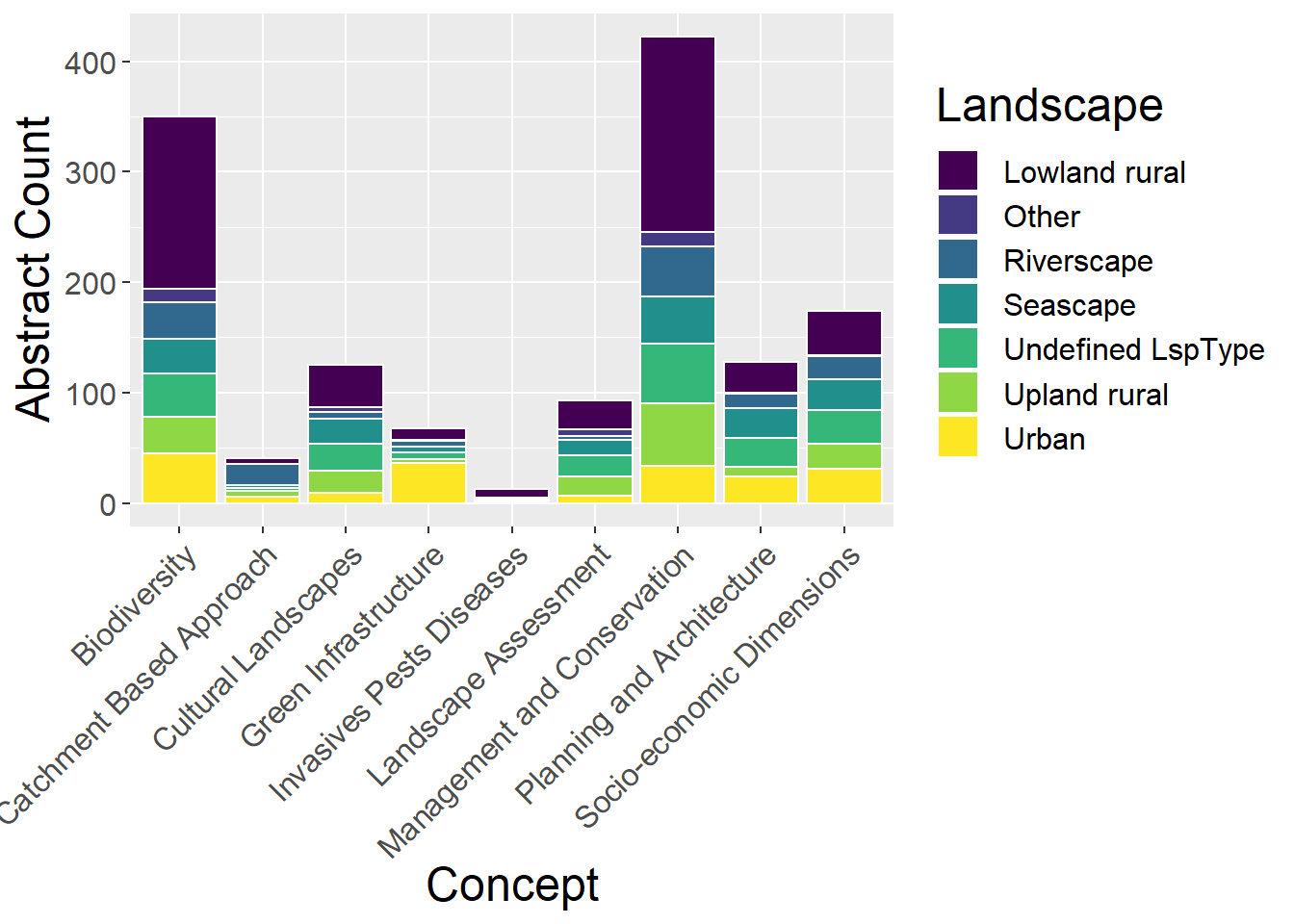

ggplot(lspCounts, aes(x=OtherC, y=prop, fill=Type)) + 
  geom_bar(stat="identity", colour="white") + 
  theme(axis.text.x = element_text(angle = 45, hjust = 1)) +
  scale_fill_viridis(discrete = TRUE) +
  labs(fill="Landscape", y = "Proportion", x="Concept")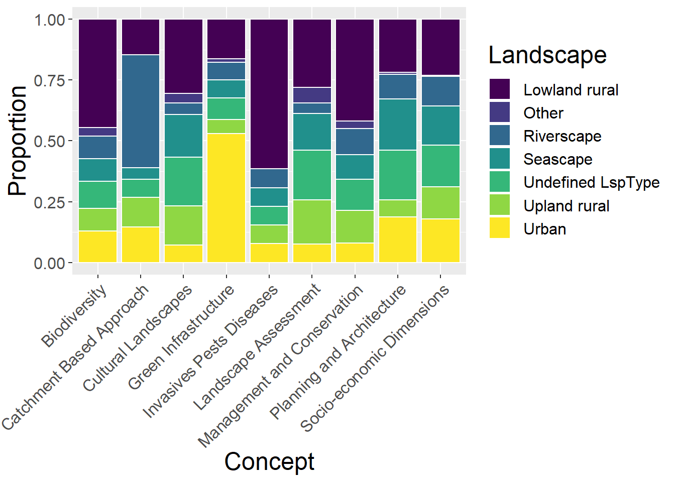

10.3.2 Without ‘Undefined LspType’ and ‘Other’ landscape types

General observations:

As above

lspCounts <- othdata %>%
  select(OtherC,`Upland rural`, `Lowland rural`, Urban, Riverscape, Seascape) %>%
  mutate(sum = rowSums(.[2:6])) %>%   #calculate total for subsquent calcultation of proportion
  gather(key = Type, value = count, -OtherC, -sum) %>%
  mutate(prop = count / sum)  #calculate proportion

othdata %>%
  select(OtherC,`Upland rural`, `Lowland rural`, Urban, Riverscape, Seascape) %>%
  mutate(Total = rowSums(.[2:6])) %>%   #calculate total
  mutate_if(is.numeric, funs(prop = ./ Total)) %>%
  mutate_at(vars(ends_with("prop")), round, 3) %>% 
  select(-Total_prop) %>%
  kable() %>%
  kable_styling() %>%
  scroll_box(width = "100%")

OtherC	Upland rural	Lowland rural	Urban	Riverscape	Seascape	Total	Upland rural_prop	Lowland rural_prop	Urban_prop	Riverscape_prop	Seascape_prop
Biodiversity	33	156	45	33	32	299	0.110	0.522	0.151	0.110	0.107
Catchment Based Approach	5	6	6	19	2	38	0.132	0.158	0.158	0.500	0.053
Cultural Landscapes	20	38	9	6	22	95	0.211	0.400	0.095	0.063	0.232
Green Infrastructure	4	11	36	5	5	61	0.066	0.180	0.590	0.082	0.082
Invasives Pests Diseases	1	8	1	1	1	12	0.083	0.667	0.083	0.083	0.083
Landscape Assessment	17	26	7	4	14	68	0.250	0.382	0.103	0.059	0.206
Management and Conservation	56	177	34	45	43	355	0.158	0.499	0.096	0.127	0.121
Planning and Architecture	9	28	24	13	27	101	0.089	0.277	0.238	0.129	0.267
Socio-economic Dimensions	23	40	31	21	28	143	0.161	0.280	0.217	0.147	0.196

ggplot(lspCounts, aes(x=OtherC, y=count, fill=Type)) + 
  geom_bar(stat="identity", colour="white") + 
  theme(axis.text.x = element_text(angle = 45, hjust = 1)) +
  scale_fill_viridis(discrete = TRUE) +
  labs(fill="Landscape", y = "Abstract Count", x="Concept")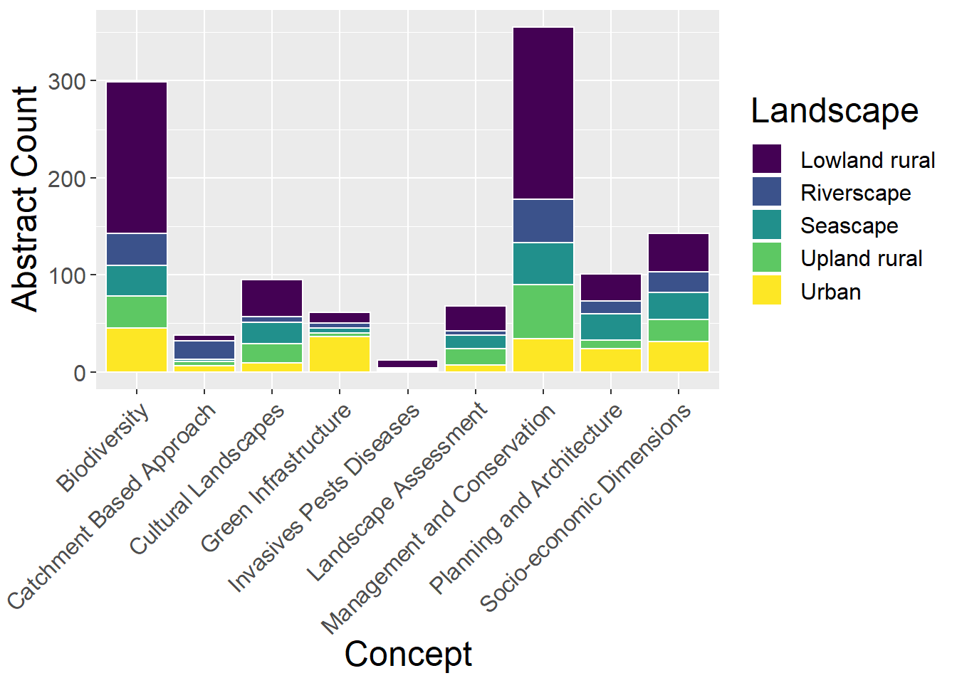

ggplot(lspCounts, aes(x=OtherC, y=prop, fill=Type)) + 
  geom_bar(stat="identity", colour="white") + 
  theme(axis.text.x = element_text(angle = 45, hjust = 1)) +
  scale_fill_viridis(discrete = TRUE) +
  labs(fill="Landscape", y = "Proportion", x="Concept")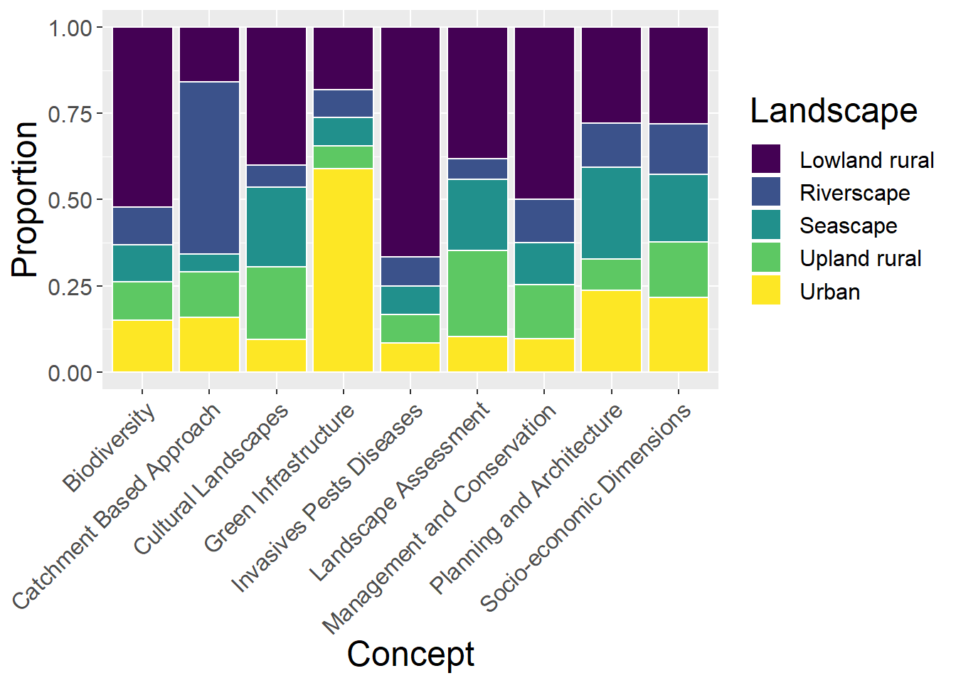

10.4 Organism

General observations

Management & Conservation studies have relatively low propotion of human studies; greatest proportion of Woodland studies
Biodiversity studies have relatively large proportion of Inverts (along with invasives)

speciesCounts <- othdata %>%
  select(OtherC, Mammals, Humans, Birds, Reptiles, Inverts, Plants, Amphibians, Fish, `Generic Habitat`,`Woodland Forests`) %>%
  mutate(sum = rowSums(.[2:11])) %>%   #calculate total for subsquent calcultation of proportion
  gather(key = Type, value = count, -OtherC, -sum) %>%
  mutate(prop = count / sum)  #calculate proportion

othdata %>%
  select(OtherC, Mammals, Humans, Birds, Reptiles, Inverts, Plants, Amphibians, Fish, `Generic Habitat`,`Woodland Forests`) %>%
  mutate(Total = rowSums(.[2:11])) %>%   #calculate total for subsquent calcultation of proportion
  mutate_if(is.numeric, funs(prop = ./ Total)) %>%
  mutate_at(vars(ends_with("prop")), round, 3) %>% 
  select(-Total_prop) %>%
  kable() %>%
  kable_styling() %>%
  scroll_box(width = "100%")

OtherC	Mammals	Humans	Birds	Reptiles	Inverts	Plants	Amphibians	Fish	Generic Habitat	Woodland Forests	Total	Mammals_prop	Humans_prop	Birds_prop	Reptiles_prop	Inverts_prop	Plants_prop	Amphibians_prop	Fish_prop	Generic Habitat_prop	Woodland Forests_prop
Biodiversity	27	20	76	4	70	62	9	9	74	64	415	0.065	0.048	0.183	0.010	0.169	0.149	0.022	0.022	0.178	0.154
Catchment Based Approach	1	6	2	1	3	4	0	0	16	4	37	0.027	0.162	0.054	0.027	0.081	0.108	0.000	0.000	0.432	0.108
Cultural Landscapes	2	39	4	1	3	4	2	1	47	20	123	0.016	0.317	0.033	0.008	0.024	0.033	0.016	0.008	0.382	0.163
Green Infrastructure	2	9	4	1	5	8	1	1	23	5	59	0.034	0.153	0.068	0.017	0.085	0.136	0.017	0.017	0.390	0.085
Invasives Pests Diseases	1	0	1	0	6	7	0	0	1	1	17	0.059	0.000	0.059	0.000	0.353	0.412	0.000	0.000	0.059	0.059
Landscape Assessment	0	11	3	0	3	3	1	0	40	8	69	0.000	0.159	0.043	0.000	0.043	0.043	0.014	0.000	0.580	0.116
Management and Conservation	23	42	83	3	42	54	3	7	100	78	435	0.053	0.097	0.191	0.007	0.097	0.124	0.007	0.016	0.230	0.179
Planning and Architecture	1	28	5	0	3	4	1	2	39	14	97	0.010	0.289	0.052	0.000	0.031	0.041	0.010	0.021	0.402	0.144
Socio-economic Dimensions	3	49	10	1	1	6	1	3	49	19	142	0.021	0.345	0.070	0.007	0.007	0.042	0.007	0.021	0.345	0.134

ggplot(speciesCounts, aes(x=OtherC, y=count, fill=Type)) + 
  geom_bar(stat="identity", colour="white") + 
  theme(axis.text.x = element_text(angle = 45, hjust = 1)) +
  scale_fill_viridis(discrete = TRUE) +
  labs(fill="Organism", y = "Abstract Count", x="Concept")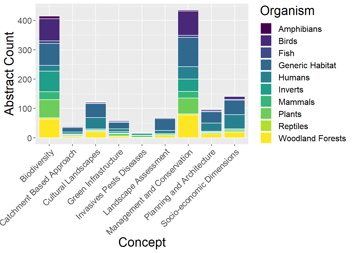

ggplot(speciesCounts, aes(x=OtherC, y=prop, fill=Type)) + 
  geom_bar(stat="identity", colour="white") + 
  theme(axis.text.x = element_text(angle = 45, hjust = 1)) +
  scale_fill_viridis(discrete = TRUE) +
  labs(fill="Organism", y = "Proportion", x="Concept")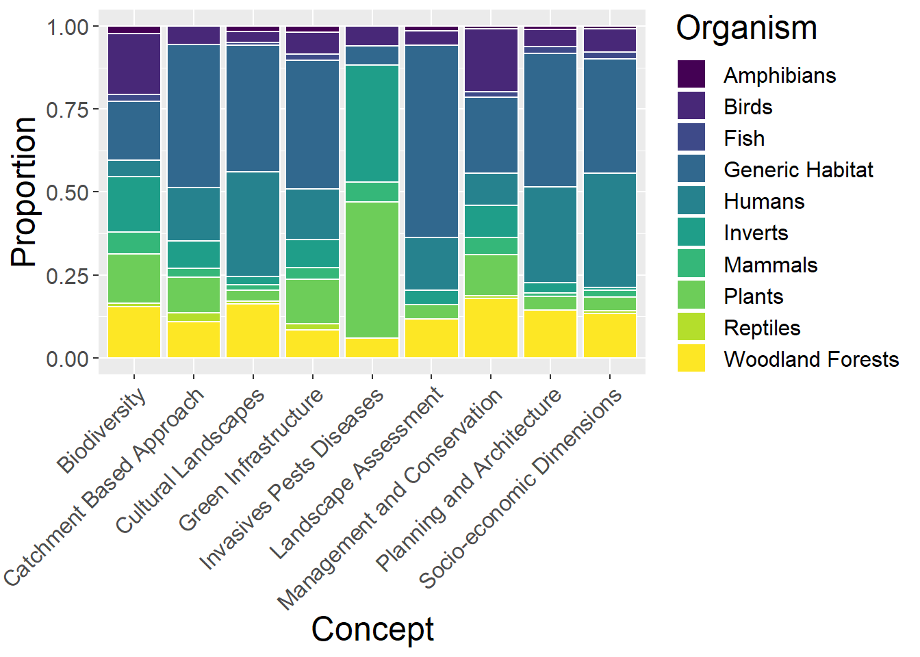

10.5 Methods

General observations:

Other than invasives, Biodiversity and Management & Conservation have greatest proportions of Empirical and lowest proportions of Theoretical

methodsCounts <- othdata %>%
  select(OtherC, Empirical, Theoretical, Qualitative, Quantitative, GIS, `Remote sensing`) %>%
  mutate(sum = rowSums(.[2:7])) %>%
  gather(key = Type, value = count, -OtherC, -sum) %>%
  mutate(prop = count / sum) 

othdata %>%
  select(OtherC, Empirical, Theoretical, Qualitative, Quantitative, GIS, `Remote sensing`) %>%
  mutate(Total = rowSums(.[2:7])) %>%
  mutate_if(is.numeric, funs(prop = ./ Total)) %>%
  mutate_at(vars(ends_with("prop")), round, 3) %>% 
  select(-Total_prop) %>%
  kable() %>%
  kable_styling() %>%
  scroll_box(width = "100%")

OtherC	Empirical	Theoretical	Qualitative	Quantitative	GIS	Remote sensing	Total	Empirical_prop	Theoretical_prop	Qualitative_prop	Quantitative_prop	GIS_prop	Remote sensing_prop
Biodiversity	170	61	48	177	71	17	544	0.312	0.112	0.088	0.325	0.131	0.031
Catchment Based Approach	8	8	7	10	8	1	42	0.190	0.190	0.167	0.238	0.190	0.024
Cultural Landscapes	27	26	56	30	23	4	166	0.163	0.157	0.337	0.181	0.139	0.024
Green Infrastructure	13	15	20	25	13	4	90	0.144	0.167	0.222	0.278	0.144	0.044
Invasives Pests Diseases	11	0	1	7	5	1	25	0.440	0.000	0.040	0.280	0.200	0.040
Landscape Assessment	17	18	24	31	23	9	122	0.139	0.148	0.197	0.254	0.189	0.074
Management and Conservation	181	85	91	176	82	16	631	0.287	0.135	0.144	0.279	0.130	0.025
Planning and Architecture	21	48	45	32	31	3	180	0.117	0.267	0.250	0.178	0.172	0.017
Socio-economic Dimensions	23	42	63	47	33	5	213	0.108	0.197	0.296	0.221	0.155	0.023

ggplot(methodsCounts, aes(x=OtherC, y=count, fill=Type)) + 
  geom_bar(stat="identity", colour="white") + 
  theme(axis.text.x = element_text(angle = 45, hjust = 1)) +
  scale_fill_viridis(discrete = TRUE) +
  labs(fill="Method", y = "Abstract Count", x="Concept")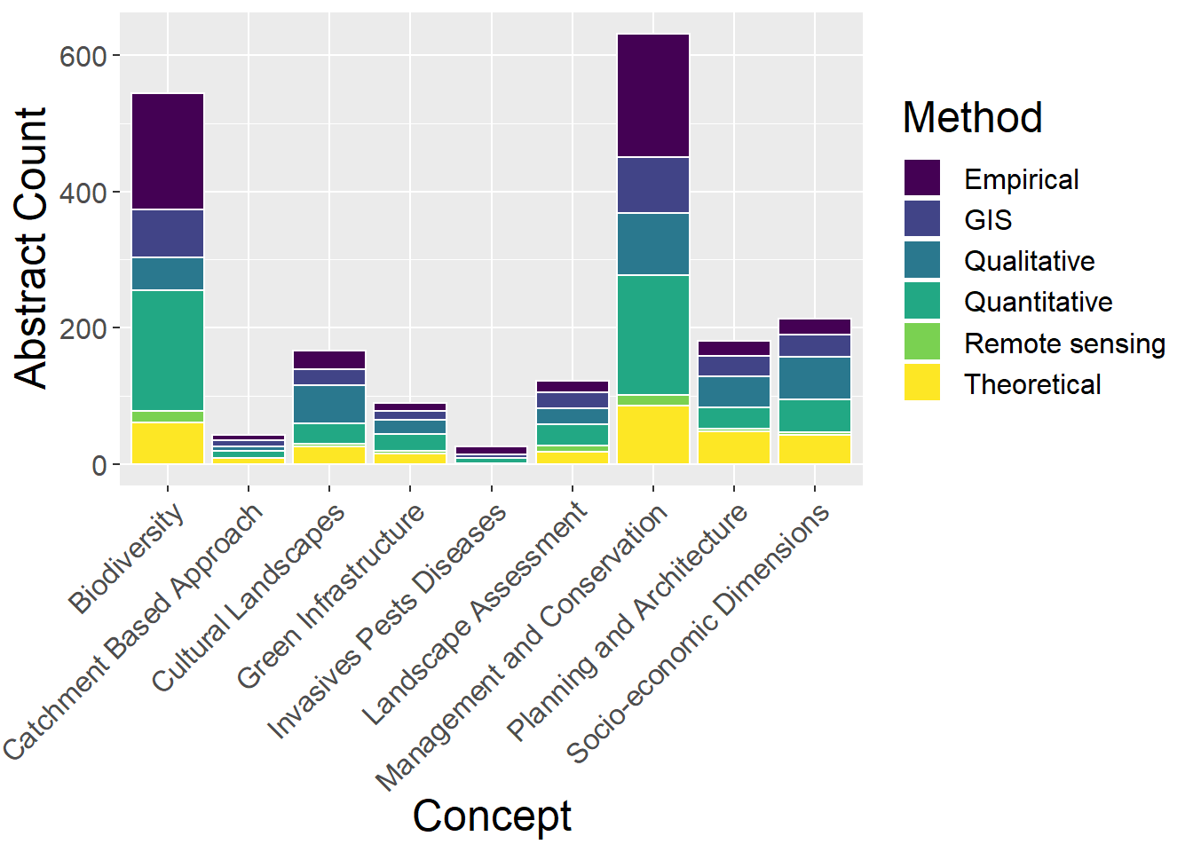

ggplot(methodsCounts, aes(x=OtherC, y=prop, fill=Type)) + 
  geom_bar(stat="identity", colour="white") + 
  theme(axis.text.x = element_text(angle = 45, hjust = 1)) +
  scale_fill_viridis(discrete = TRUE) +
  labs(fill="Method", y = "Proportion", x="Concept")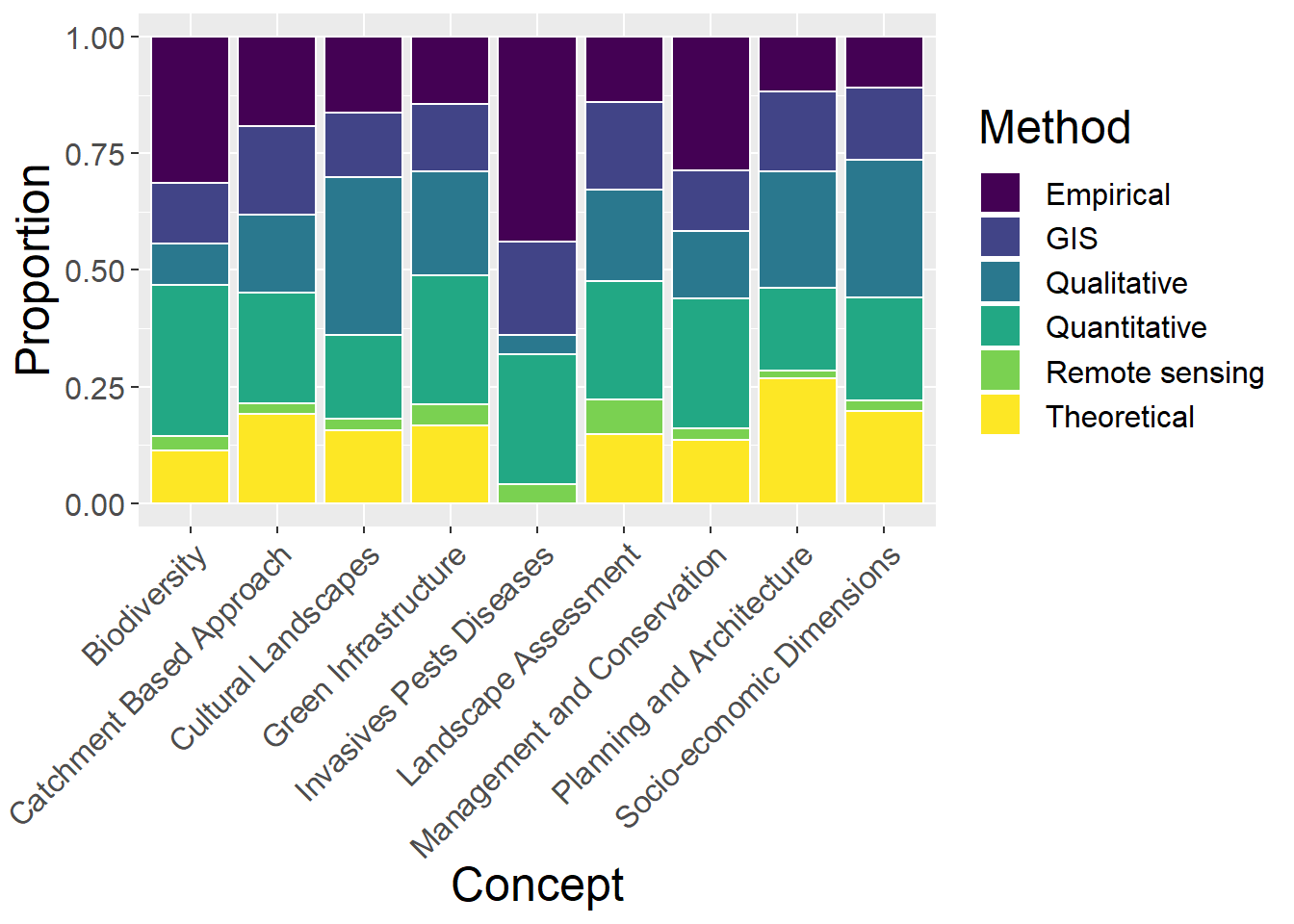

10.6 Spatial Extent

General observations:

spatialCounts <- othdata %>%
  select(OtherC, Micro, Mini, Local, Regional, National, Continental, Global,`Undefined Extent`) %>%
  mutate(sum = rowSums(.[2:9])) %>%
  gather(key = Type, value = count, -OtherC, -sum) %>%
  mutate(prop = count / sum) 

othdata %>%
  select(OtherC, Micro, Mini, Local, Regional, National, Continental, Global,`Undefined Extent`) %>%
  mutate(Total = rowSums(.[2:9])) %>%
  mutate_if(is.numeric, funs(prop = ./ Total)) %>%
  mutate_at(vars(ends_with("prop")), round, 3) %>% 
  select(-Total_prop) %>%
  kable() %>%
  kable_styling() %>%
  scroll_box(width = "100%")

OtherC	Micro	Mini	Local	Regional	National	Continental	Global	Undefined Extent	Total	Micro_prop	Mini_prop	Local_prop	Regional_prop	National_prop	Continental_prop	Global_prop	Undefined Extent_prop
Biodiversity	17	49	81	70	54	7	6	43	327	0.052	0.150	0.248	0.214	0.165	0.021	0.018	0.131
Catchment Based Approach	1	3	16	8	3	0	0	4	35	0.029	0.086	0.457	0.229	0.086	0.000	0.000	0.114
Cultural Landscapes	0	7	34	37	19	9	1	14	121	0.000	0.058	0.281	0.306	0.157	0.074	0.008	0.116
Green Infrastructure	3	10	22	13	6	1	1	6	62	0.048	0.161	0.355	0.210	0.097	0.016	0.016	0.097
Invasives Pests Diseases	3	5	1	2	1	2	0	0	14	0.214	0.357	0.071	0.143	0.071	0.143	0.000	0.000
Landscape Assessment	2	4	14	19	22	6	2	11	80	0.025	0.050	0.175	0.238	0.275	0.075	0.025	0.138
Management and Conservation	12	41	109	89	75	16	7	50	399	0.030	0.103	0.273	0.223	0.188	0.040	0.018	0.125
Planning and Architecture	2	8	43	28	28	2	3	22	136	0.015	0.059	0.316	0.206	0.206	0.015	0.022	0.162
Socio-economic Dimensions	1	7	47	38	25	6	2	25	151	0.007	0.046	0.311	0.252	0.166	0.040	0.013	0.166

tfactor_order <- c('Micro', 'Mini', 'Local', 'Regional', 'National', 'Continental', 'Global','Undefined Extent')
tfactor_labels <- c('Micro', 'Mini', 'Local', 'Regional', 'National', 'Continental', 'Global','Undefined')

ggplot(spatialCounts, aes(x=OtherC, y=count, fill=factor(Type, level=tfactor_order))) + 
  geom_bar(stat="identity", colour="white") + 
  theme(axis.text.x = element_text(angle = 45, hjust = 1)) +
  scale_fill_viridis(discrete = TRUE) +
  labs(fill="Spatial", y = "Abstract Count", x="Concept")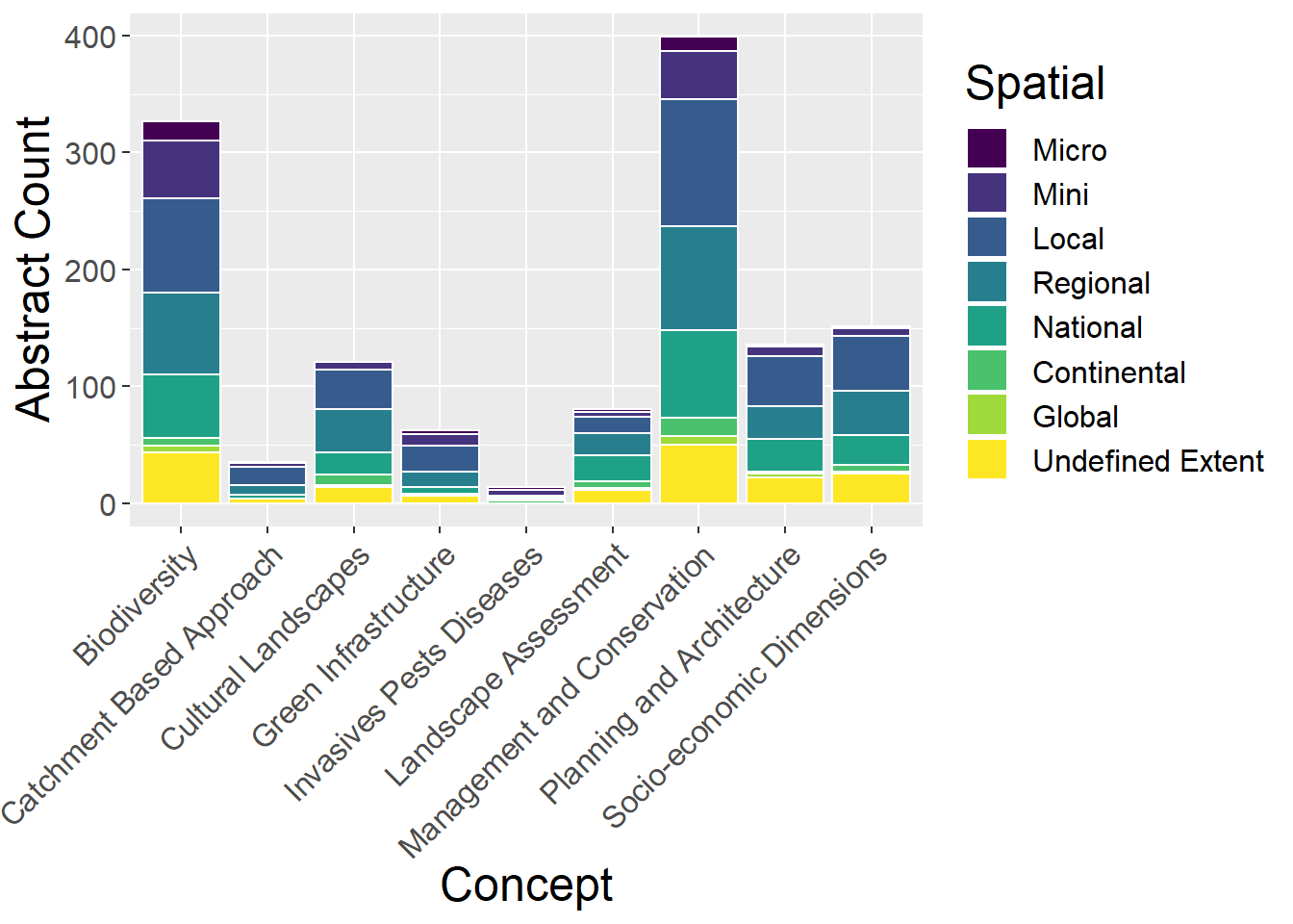

ggplot(spatialCounts, aes(x=OtherC, y=prop, fill=factor(Type, level=tfactor_order))) + 
  geom_bar(stat="identity", colour="white") + 
  theme(axis.text.x = element_text(angle = 45, hjust = 1)) +
  scale_fill_viridis(discrete = TRUE) +
  labs(fill="Spatial", y = "Proportion", x="Concept")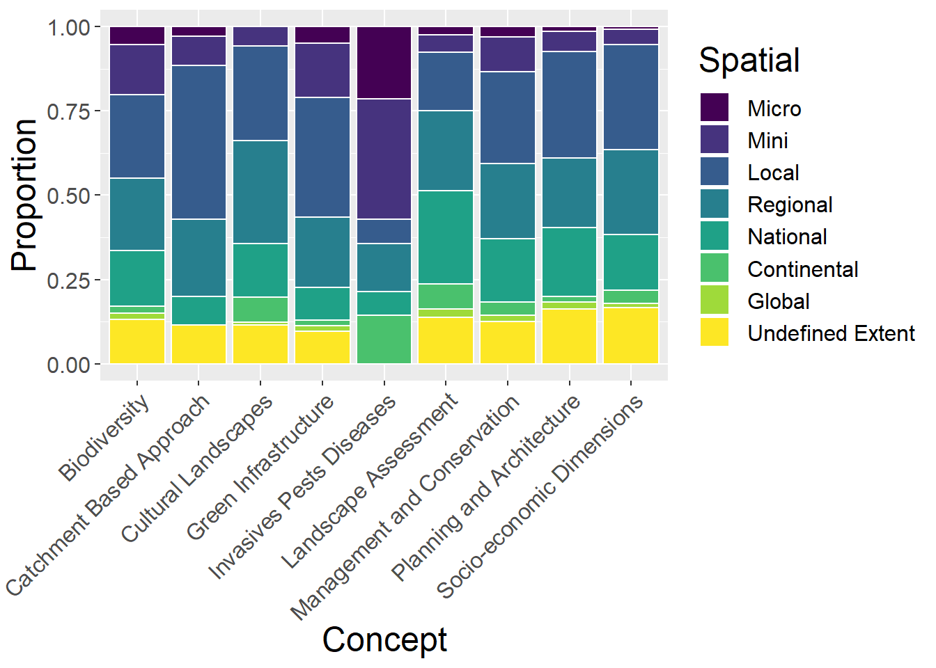

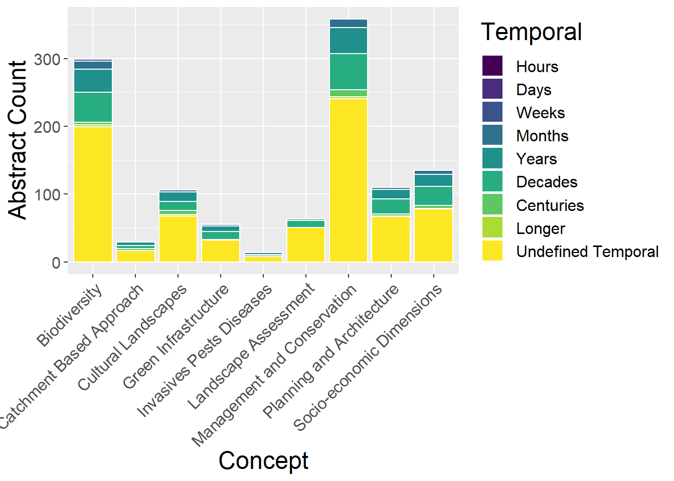
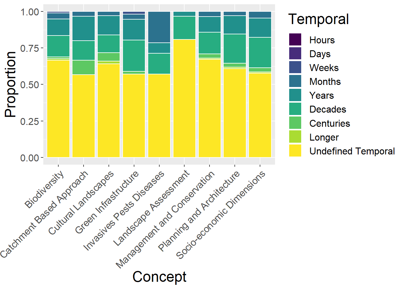
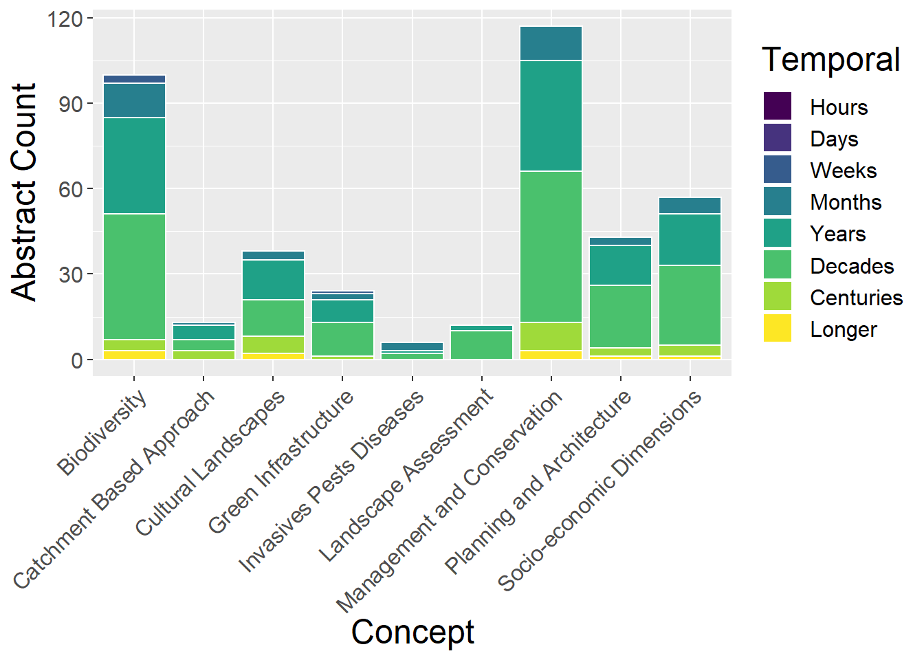
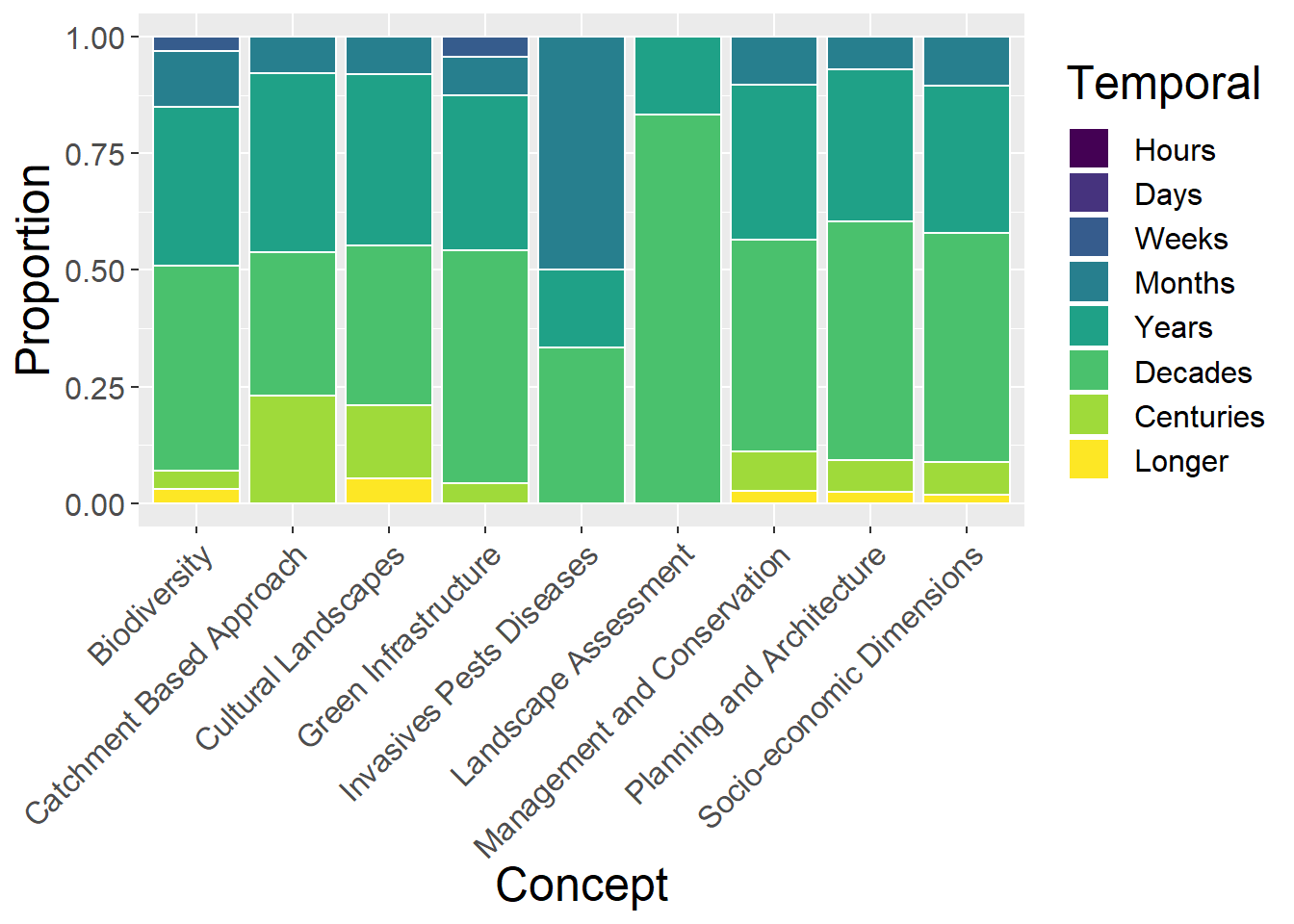
10.7 Temporal Extent

10.7.1 With undefined

General observations:

No obvious patterns

OtherC	Weeks	Months	Years	Decades	Centuries	Longer	Undefined Temporal	Total	Weeks_prop	Months_prop	Years_prop	Decades_prop	Centuries_prop	Longer_prop	Undefined Temporal_prop
Biodiversity	3	12	34	44	4	3	199	299	0.010	0.040	0.114	0.147	0.013	0.010	0.666
Catchment Based Approach	0	1	5	4	3	0	17	30	0.000	0.033	0.167	0.133	0.100	0.000	0.567
Cultural Landscapes	0	3	14	13	6	2	68	106	0.000	0.028	0.132	0.123	0.057	0.019	0.642
Green Infrastructure	1	2	8	12	1	0	32	56	0.018	0.036	0.143	0.214	0.018	0.000	0.571
Invasives Pests Diseases	0	3	1	2	0	0	8	14	0.000	0.214	0.071	0.143	0.000	0.000	0.571
Landscape Assessment	0	0	2	10	0	0	51	63	0.000	0.000	0.032	0.159	0.000	0.000	0.810
Management and Conservation	0	12	39	53	10	3	241	358	0.000	0.034	0.109	0.148	0.028	0.008	0.673
Planning and Architecture	0	3	14	22	3	1	67	110	0.000	0.027	0.127	0.200	0.027	0.009	0.609
Socio-economic Dimensions	0	6	18	28	4	1	78	135	0.000	0.044	0.133	0.207	0.030	0.007	0.578

10.7.2 Without Undefined

No obvious patterns

OtherC	Weeks	Months	Years	Decades	Centuries	Longer	Total	Weeks_prop	Months_prop	Years_prop	Decades_prop	Centuries_prop	Longer_prop
Biodiversity	3	12	34	44	4	3	100	0.030	0.120	0.340	0.440	0.040	0.030
Catchment Based Approach	0	1	5	4	3	0	13	0.000	0.077	0.385	0.308	0.231	0.000
Cultural Landscapes	0	3	14	13	6	2	38	0.000	0.079	0.368	0.342	0.158	0.053
Green Infrastructure	1	2	8	12	1	0	24	0.042	0.083	0.333	0.500	0.042	0.000
Invasives Pests Diseases	0	3	1	2	0	0	6	0.000	0.500	0.167	0.333	0.000	0.000
Landscape Assessment	0	0	2	10	0	0	12	0.000	0.000	0.167	0.833	0.000	0.000
Management and Conservation	0	12	39	53	10	3	117	0.000	0.103	0.333	0.453	0.085	0.026
Planning and Architecture	0	3	14	22	3	1	43	0.000	0.070	0.326	0.512	0.070	0.023
Socio-economic Dimensions	0	6	18	28	4	1	57	0.000	0.105	0.316	0.491	0.070	0.018

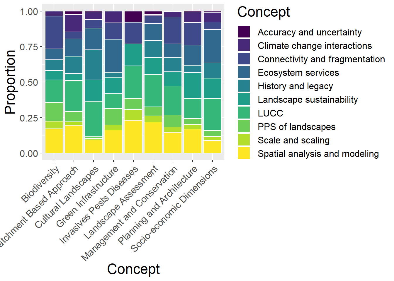
10.8 Concepts

General observations:

Biodiversity and Management & Conservation have similar proportions; both with relatively large proportions of connectivity and fragmentation

conceptCounts <- othdata %>%
  select(OtherC, `PPS of landscapes`,
`Connectivity and fragmentation`, `Scale and scaling`,`Spatial analysis and modeling`,LUCC,`History and legacy`,`Climate change interactions`,`Ecosystem services`,`Landscape sustainability`,`Accuracy and uncertainty`
) %>%
  mutate(sum = rowSums(.[2:11])) %>%
  gather(key = Type, value = count, -OtherC, -sum) %>%
  mutate(prop = count / sum) 


othdata %>%
  select(OtherC, `PPS of landscapes`,
`Connectivity and fragmentation`, `Scale and scaling`,`Spatial analysis and modeling`,LUCC,`History and legacy`,`Climate change interactions`,`Ecosystem services`,`Landscape sustainability`,`Accuracy and uncertainty`
) %>%
  mutate(Total = rowSums(.[2:11])) %>%
  mutate_if(is.numeric, funs(prop = ./ Total)) %>%
  mutate_at(vars(ends_with("prop")), round, 3) %>% 
  select(-Total_prop) %>%
  kable() %>%
  kable_styling() %>%
  scroll_box(width = "100%")

OtherC	PPS of landscapes	Connectivity and fragmentation	Scale and scaling	Spatial analysis and modeling	LUCC	History and legacy	Climate change interactions	Ecosystem services	Landscape sustainability	Accuracy and uncertainty	Total	PPS of landscapes_prop	Connectivity and fragmentation_prop	Scale and scaling_prop	Spatial analysis and modeling_prop	LUCC_prop	History and legacy_prop	Climate change interactions_prop	Ecosystem services_prop	Landscape sustainability_prop	Accuracy and uncertainty_prop
Biodiversity	59	104	24	77	71	34	15	35	30	0	449	0.131	0.232	0.053	0.171	0.158	0.076	0.033	0.078	0.067	0.000
Catchment Based Approach	3	2	1	8	9	5	5	5	2	1	41	0.073	0.049	0.024	0.195	0.220	0.122	0.122	0.122	0.049	0.024
Cultural Landscapes	2	11	2	17	46	39	10	28	28	1	184	0.011	0.060	0.011	0.092	0.250	0.212	0.054	0.152	0.152	0.005
Green Infrastructure	10	10	3	14	9	3	7	20	10	0	86	0.116	0.116	0.035	0.163	0.105	0.035	0.081	0.233	0.116	0.000
Invasives Pests Diseases	1	2	1	3	3	0	0	0	2	1	13	0.077	0.154	0.077	0.231	0.231	0.000	0.000	0.000	0.154	0.077
Landscape Assessment	6	5	4	20	21	11	1	11	11	2	92	0.065	0.054	0.043	0.217	0.228	0.120	0.011	0.120	0.120	0.022
Management and Conservation	44	97	18	75	104	51	20	49	52	1	511	0.086	0.190	0.035	0.147	0.204	0.100	0.039	0.096	0.102	0.002
Planning and Architecture	8	30	6	32	27	10	14	27	34	1	189	0.042	0.159	0.032	0.169	0.143	0.053	0.074	0.143	0.180	0.005
Socio-economic Dimensions	10	13	7	21	54	26	16	56	34	2	239	0.042	0.054	0.029	0.088	0.226	0.109	0.067	0.234	0.142	0.008

ggplot(conceptCounts, aes(x=OtherC, y=count, fill=Type)) + 
  geom_bar(stat="identity", colour="white") + 
  theme(axis.text.x = element_text(angle = 45, hjust = 1)) +
  scale_fill_viridis(discrete = TRUE) +
  labs(fill="Concept", y = "Abstract Count", x="Concept")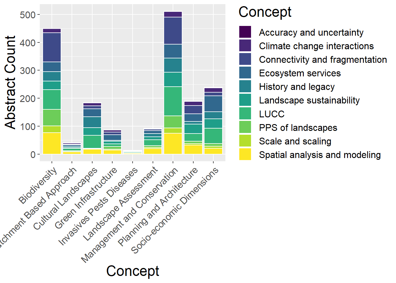

ggplot(conceptCounts, aes(x=OtherC, y=prop, fill=Type)) + 
  geom_bar(stat="identity", colour="white") + 
  theme(axis.text.x = element_text(angle = 45, hjust = 1)) +
  scale_fill_viridis(discrete = TRUE) +
  labs(fill="Concept", y = "Proportion", x="Concept")