Chapter 4 Analysis by Landscape Type

Bar charts and tables to examine how contribution to conferences have changed over time.

4.1 Total Conference Contributions

#spec(cpdata)

lspdata <- cpdata %>%
  select_if(is.numeric) %>%
  gather(key = LspType, value = count, `Upland rural`:Other) %>%
  filter(count > 0) %>%
  group_by(`LspType`) %>%
  summarise_all(sum, na.rm=T) 

General observations:

• Lowland rural dominate, followed by ‘undefined’ and Upland rural

lspdata %>%
  select(LspType, count) %>%
  mutate(prop = count/sum(count)) %>%
  mutate(prop = round(prop,3)) %>% 
  kable() %>%
  kable_styling() %>%
  scroll_box(width = "100%")

LspType	count	prop
Lowland rural	363	0.406
Other	26	0.029
Riverscape	96	0.108
Seascape	68	0.076
Undefined LspType	136	0.152
Upland rural	114	0.128
Urban	90	0.101

ggplot(lspdata, aes(x=LspType, y=count)) + 
  geom_bar(stat="identity") + 
  geom_text(aes(x=LspType, y=max(count), label = paste0(round(100*count / sum(count),1), "%"), vjust=-0.25)) +
  theme(axis.text.x = element_text(angle = 30, hjust = 1))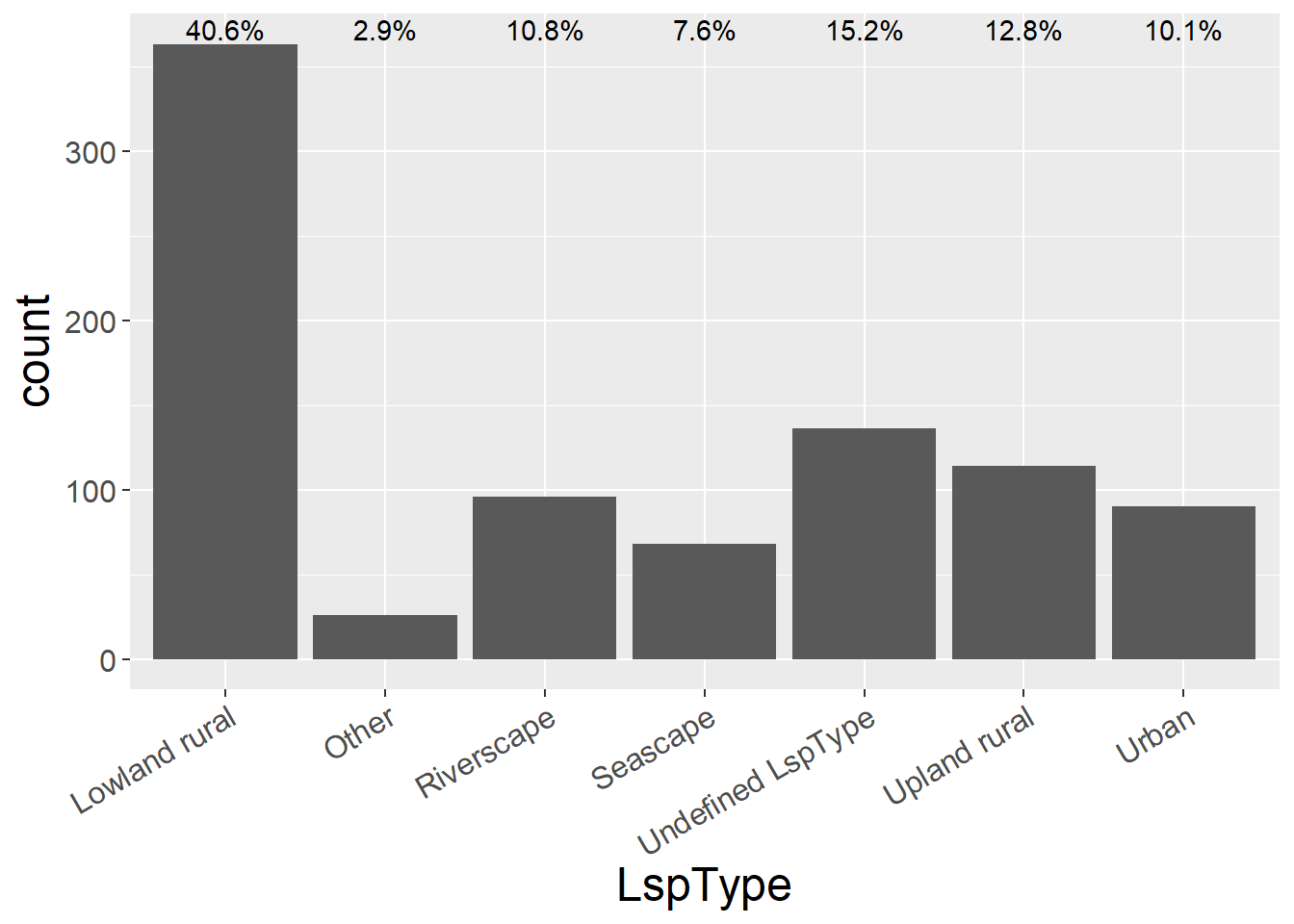

4.2 Author Affiliation

General observations:

• Academic are majority of all landscape types, with possible exception of Upland rural (Government?)

authorCounts <- lspdata %>%
  select(LspType,Academic, Government,NGO,Business,Private) %>%
  mutate(sum = rowSums(.[2:6])) %>%   #calculate total for subsquent calcultation of proportion
  gather(key = Type, value = count, -LspType, -sum) %>%
  mutate(prop = count / sum)  #calculate proportion

ggplot(authorCounts, aes(x=LspType, y=count, fill=Type)) + geom_bar(stat="identity", colour="white") +
  scale_fill_viridis(discrete = TRUE) +
  theme(axis.text.x = element_text(angle = 30, hjust = 1)) +
  labs(fill="Affiliation", y = "Abstract Count")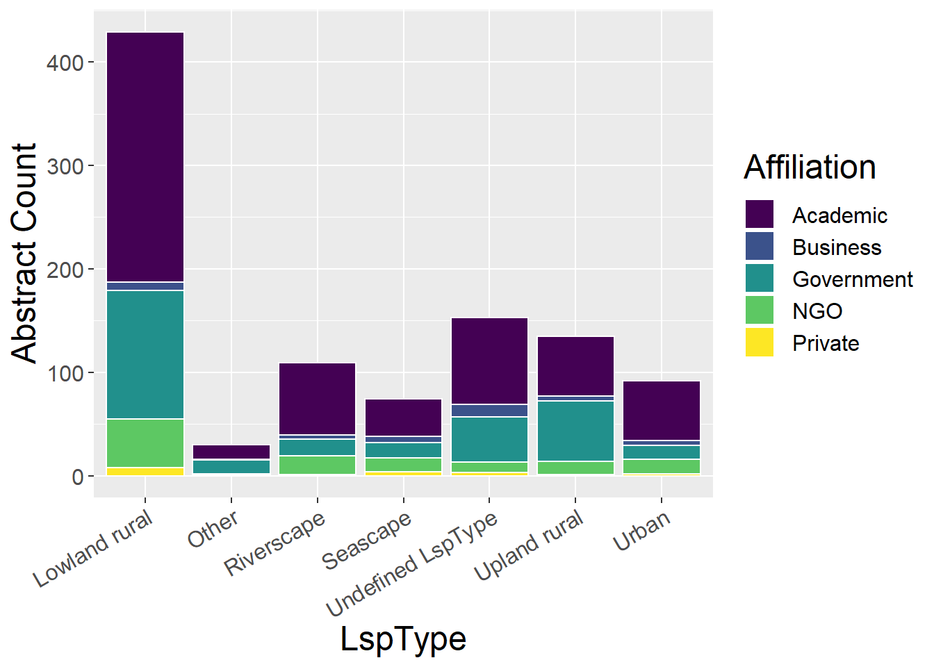

ggplot(authorCounts, aes(x=LspType, y=prop, fill=Type)) + geom_bar(stat="identity", colour="white") +
  scale_fill_viridis(discrete = TRUE) +
  theme(axis.text.x = element_text(angle = 30, hjust = 1)) +
  labs(fill="Affiliation", y = "Proportion")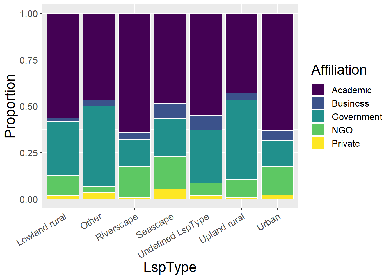

4.3 Organism

General observations:

• Animal types quite evenly distributed across Lowland rural
• Humans are large contributor to seascape studies (possibly by absolute number as well as relative)
• Generic habitat is large contributor across all landscape types

sppCounts <- lspdata %>%
  select(LspType,Mammals, Humans, Birds, Reptiles, Inverts, Plants, Amphibians, Fish, `Generic Habitat`,`Woodland Forests`) %>%
  mutate(sum = rowSums(.[2:11])) %>%   #calculate total for subsquent calcultation of proportion
  gather(key = Type, value = count, -LspType, -sum) %>%
  mutate(prop = count / sum)  #calculate proportion

ggplot(sppCounts, aes(x=LspType, y=count, fill=Type)) + geom_bar(stat="identity", colour="white") +
  scale_fill_viridis(discrete = TRUE) +
  theme(axis.text.x = element_text(angle = 30, hjust = 1)) +
  labs(fill="Organism", y = "Abstract Count")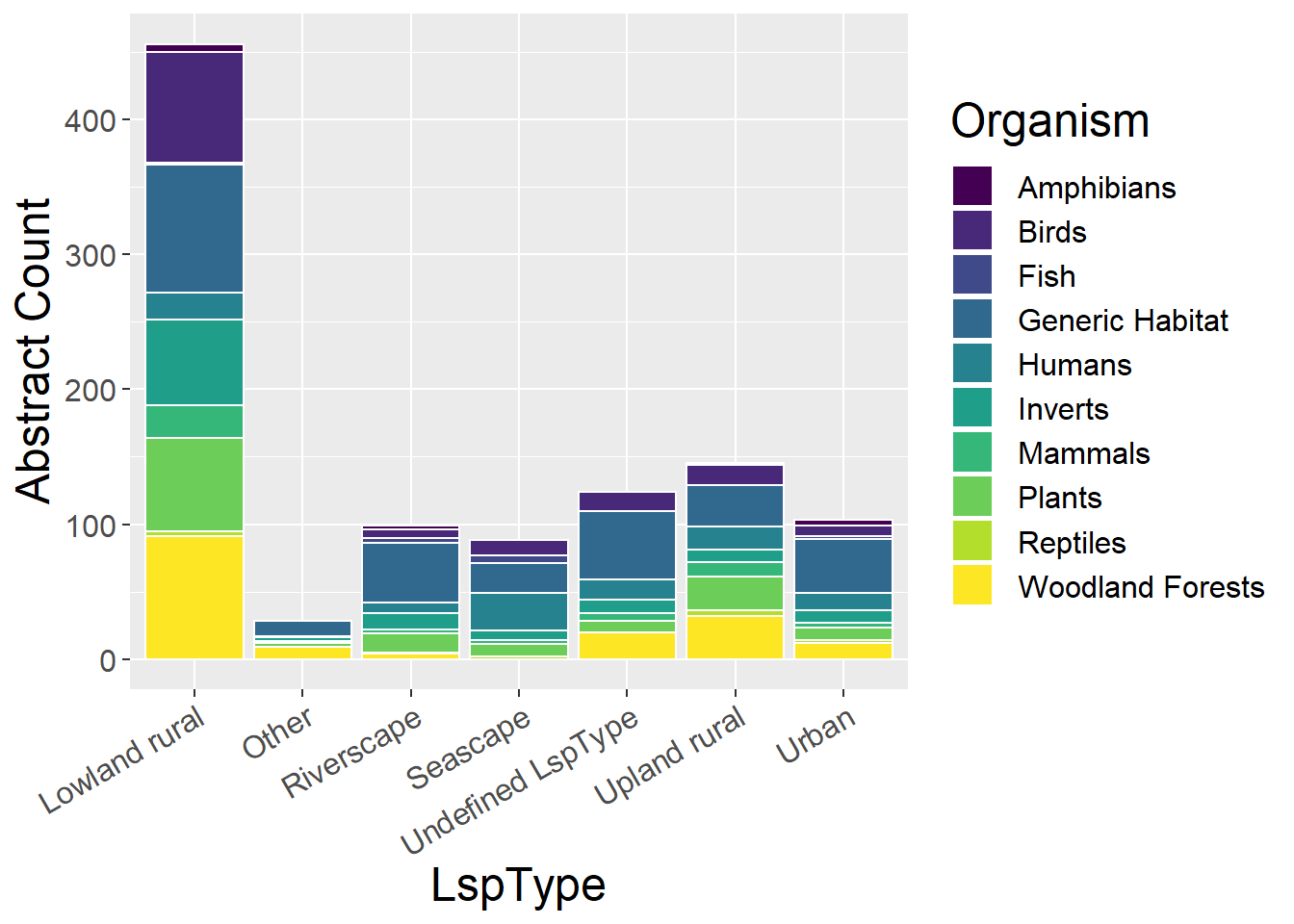

ggplot(sppCounts, aes(x=LspType, y=prop, fill=Type)) + geom_bar(stat="identity", colour="white") +
  scale_fill_viridis(discrete = TRUE) +
  theme(axis.text.x = element_text(angle = 30, hjust = 1)) +
  labs(fill="Organism", y = "Proportion")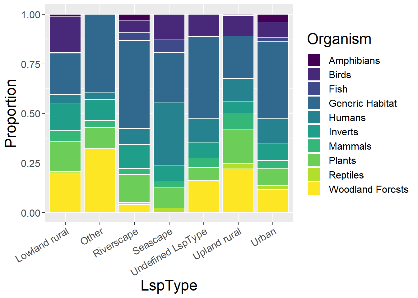

4.4 Methods

General observations:

• ‘Undefined landscape’ studies are largely theoretical
• Lowland rural largely studies using empirical and quantitative methods
• Seascape studies have largest proportion of qualitative methods

methodsCounts <- lspdata %>%
  select(LspType,Empirical, Theoretical, Qualitative, Quantitative, GIS, `Remote sensing`) %>%
  mutate(sum = rowSums(.[2:7])) %>%   #calculate total for subsquent calcultation of proportion
  gather(key = Type, value = count, -LspType, -sum) %>%
  mutate(prop = count / sum)  #calculate proportion

ggplot(methodsCounts, aes(x=LspType, y=count, fill=Type)) + geom_bar(stat="identity", colour="white") +
  scale_fill_viridis(discrete = TRUE) +
  theme(axis.text.x = element_text(angle = 30, hjust = 1)) +
  labs(fill="Method", y = "Abstract Count")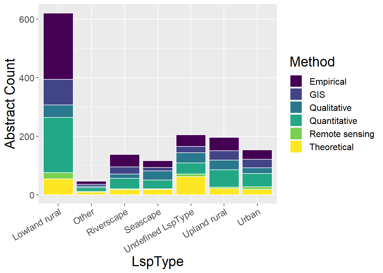

ggplot(methodsCounts, aes(x=LspType, y=prop, fill=Type)) + geom_bar(stat="identity", colour="white") +
  scale_fill_viridis(discrete = TRUE) +
  theme(axis.text.x = element_text(angle = 30, hjust = 1)) +
  labs(fill="Method", y = "Proportion")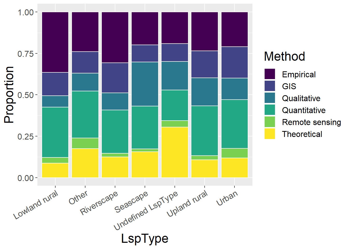

4.5 Spatial Extent

General observations:

• Urban landscape studies are dominated by Local scale analysis
• Upland rural have larger proportion of national studies than Lowland rural

spatialCounts <- lspdata %>%
  select(LspType,Micro, Mini, Local, Regional, National, Continental, Global,`Undefined Extent`) %>%
  mutate(sum = rowSums(.[2:9])) %>%   #calculate total for subsquent calcultation of proportion
  gather(key = Type, value = count, -LspType, -sum) %>%
  mutate(prop = count / sum)  #calculate proportion

factor_order <- c('Micro', 'Mini', 'Local', 'Regional', 'National', 'Continental', 'Global','Undefined Extent')
factor_labels <- c('Micro', 'Mini', 'Local', 'Regional', 'National', 'Continental', 'Global','Undefined')

ggplot(spatialCounts, aes(x=LspType, y=count, fill=factor(Type, level=factor_order))) + geom_bar(stat="identity", colour="white") +
  scale_fill_viridis(discrete = TRUE) +
  theme(axis.text.x = element_text(angle = 30, hjust = 1)) +
  labs(fill="Extent", y = "Abstract Count")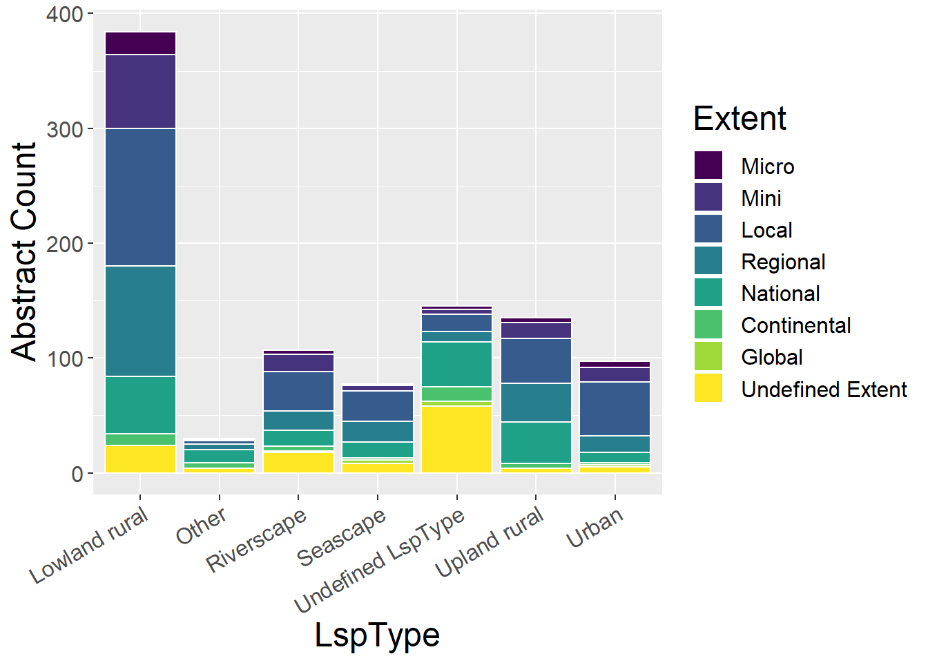

ggplot(spatialCounts, aes(x=LspType, y=prop, fill=factor(Type, level=factor_order))) + geom_bar(stat="identity", colour="white") +
  scale_fill_viridis(discrete = TRUE) +
  theme(axis.text.x = element_text(angle = 30, hjust = 1)) +
  labs(fill="Extent", y = "Proportion")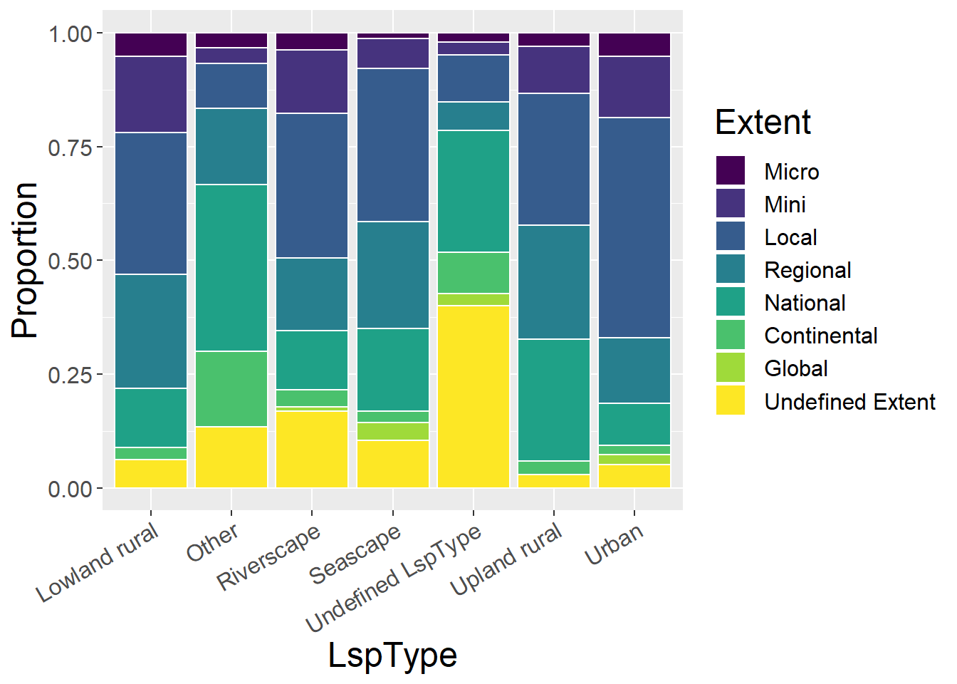

4.6 Temporal Extent

General observations:

• Upland have greatest proportion of Decadal studies
• Urban have greatest proportion of Monthly studies

temporalCounts <- lspdata %>%
  select(LspType,Hours, Days, Weeks, Months, Years, Decades, Centuries, Longer, `Undefined Temporal`) %>%
  mutate(sum = rowSums(.[2:10])) %>%   #calculate total for subsquent calcultation of proportion
  gather(key = Type, value = count, -LspType, -sum) %>%
  mutate(prop = count / sum)  #calculate proportion

tfactor_order <- c('Hours', 'Days', 'Weeks', 'Months', 'Years', 'Decades', 'Centuries', 'Longer', 'Undefined Temporal')
tfactor_labels <- c('Hours', 'Days', 'Weeks', 'Months', 'Years', 'Decades', 'Centuries', 'Longer', 'Undefined')

ggplot(temporalCounts, aes(x=LspType, y=count, fill=factor(Type, level=tfactor_order))) + geom_bar(stat="identity", colour="white") +
  scale_fill_viridis(discrete = TRUE) +
  theme(axis.text.x = element_text(angle = 30, hjust = 1)) +
  labs(fill="Extent", y = "Abstract Count")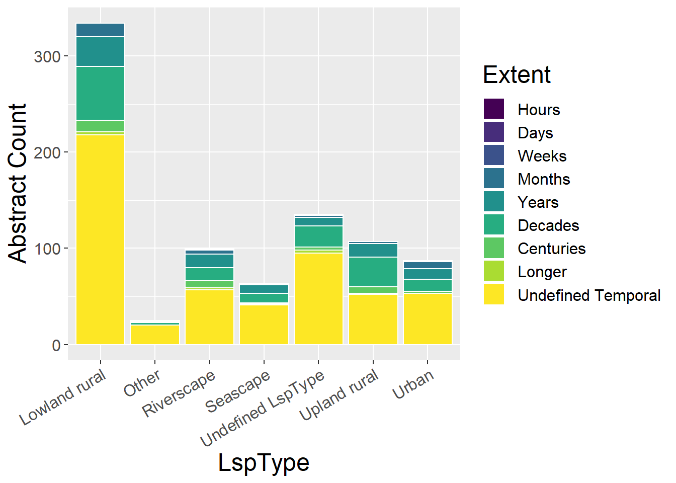

ggplot(temporalCounts, aes(x=LspType, y=prop, fill=factor(Type, level=tfactor_order))) + geom_bar(stat="identity", colour="white") +
  scale_fill_viridis(discrete = TRUE) +
  theme(axis.text.x = element_text(angle = 30, hjust = 1)) +
  labs(fill="Extent", y = "Proportion")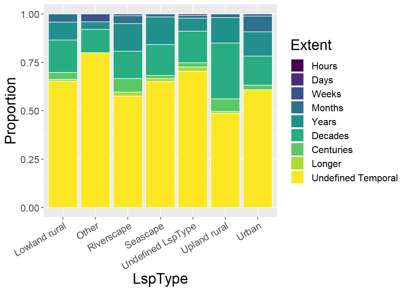

4.7 Concepts

General observations:

• Upland have greatest proportion of LUCC studies
• Seascape have greatest proportion of climate change studies

conceptCounts <- lspdata %>%
  select(`LspType`,`PPS of landscapes`,
`Connectivity and fragmentation`, `Scale and scaling`,`Spatial analysis and modeling`,LUCC,`History and legacy`,`Climate change interactions`,`Ecosystem services`,`Landscape sustainability`,`Accuracy and uncertainty`) %>%
  mutate(sum = rowSums(.[2:11])) %>%   #calculate total for subsquent calcultation of proportion
  gather(key = Type, value = count, -`LspType`, -sum) %>%
  mutate(prop = count / sum)  #calculate proportion

ggplot(conceptCounts, aes(x=`LspType`, y=count, fill=Type)) + geom_bar(stat="identity", colour="white") +
  scale_fill_viridis(discrete = TRUE) +
  theme(axis.text.x = element_text(angle = 30, hjust = 1)) +
  labs(fill="Concept", y = "Abstract Count")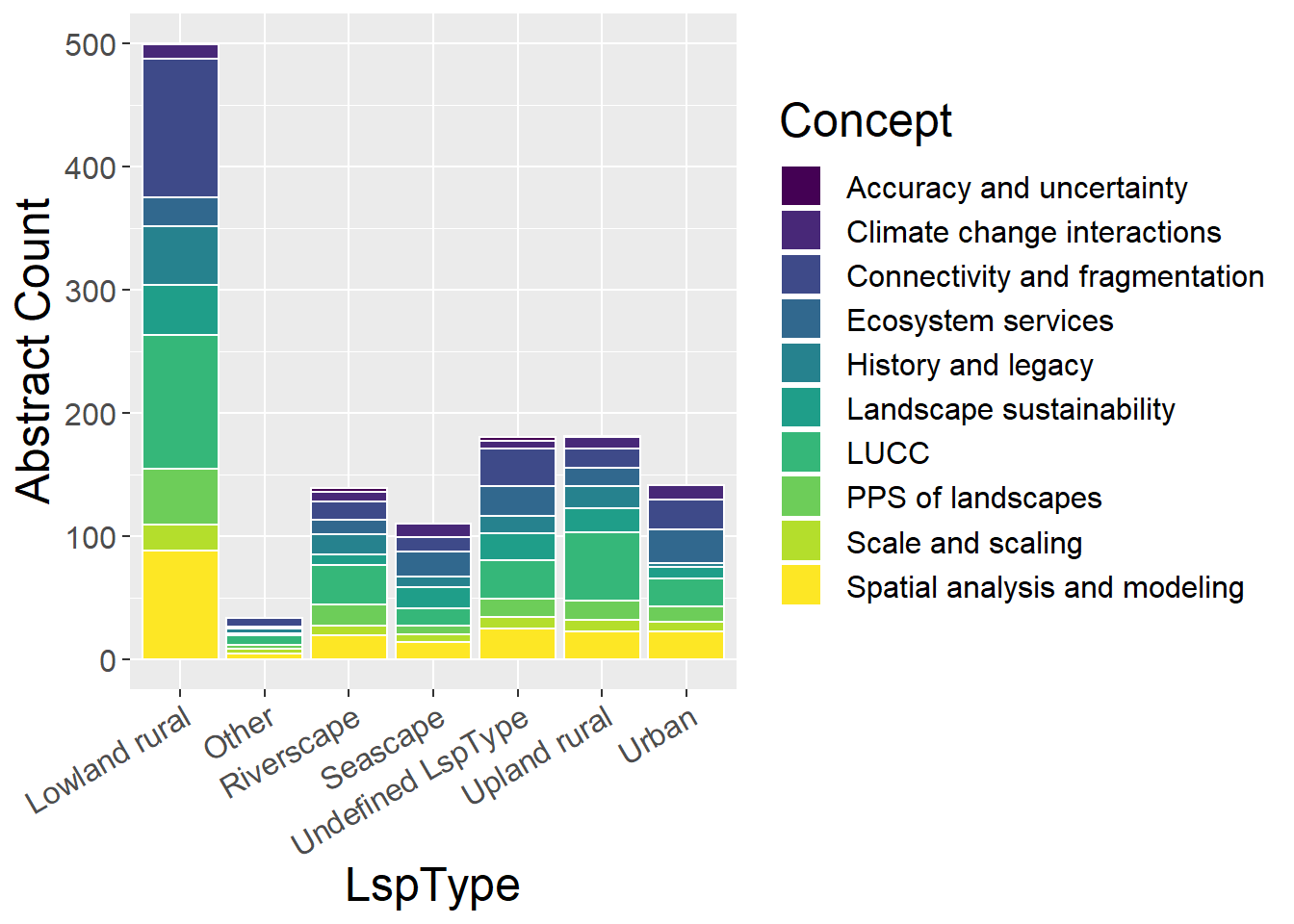

ggplot(conceptCounts, aes(x=`LspType`, y=prop, fill=Type)) + geom_bar(stat="identity", colour="white") +
  scale_fill_viridis(discrete = TRUE) +
  theme(axis.text.x = element_text(angle = 30, hjust = 1)) +
  labs(fill="Concept", y = "Proportion")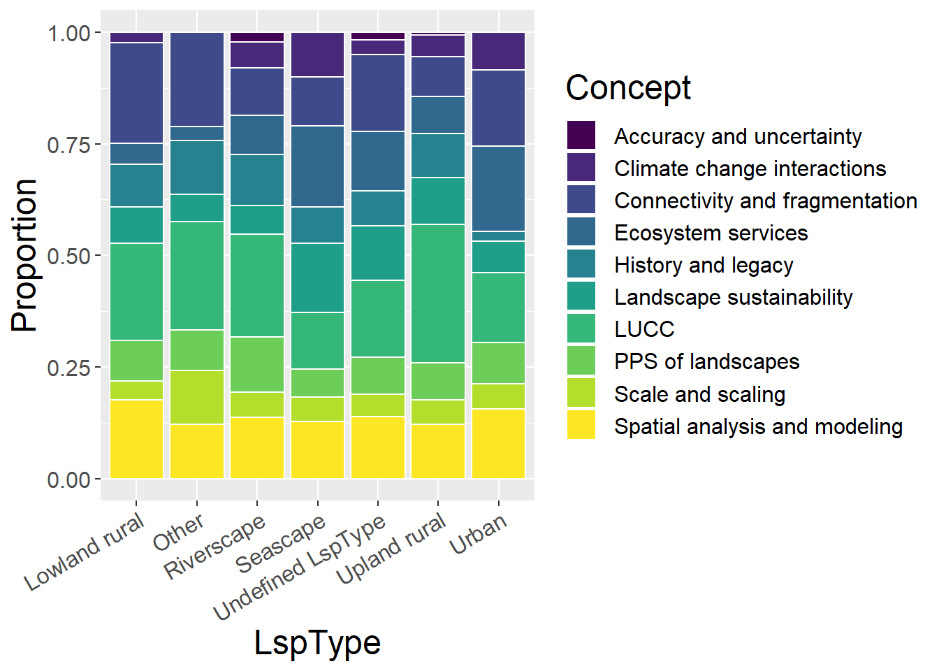

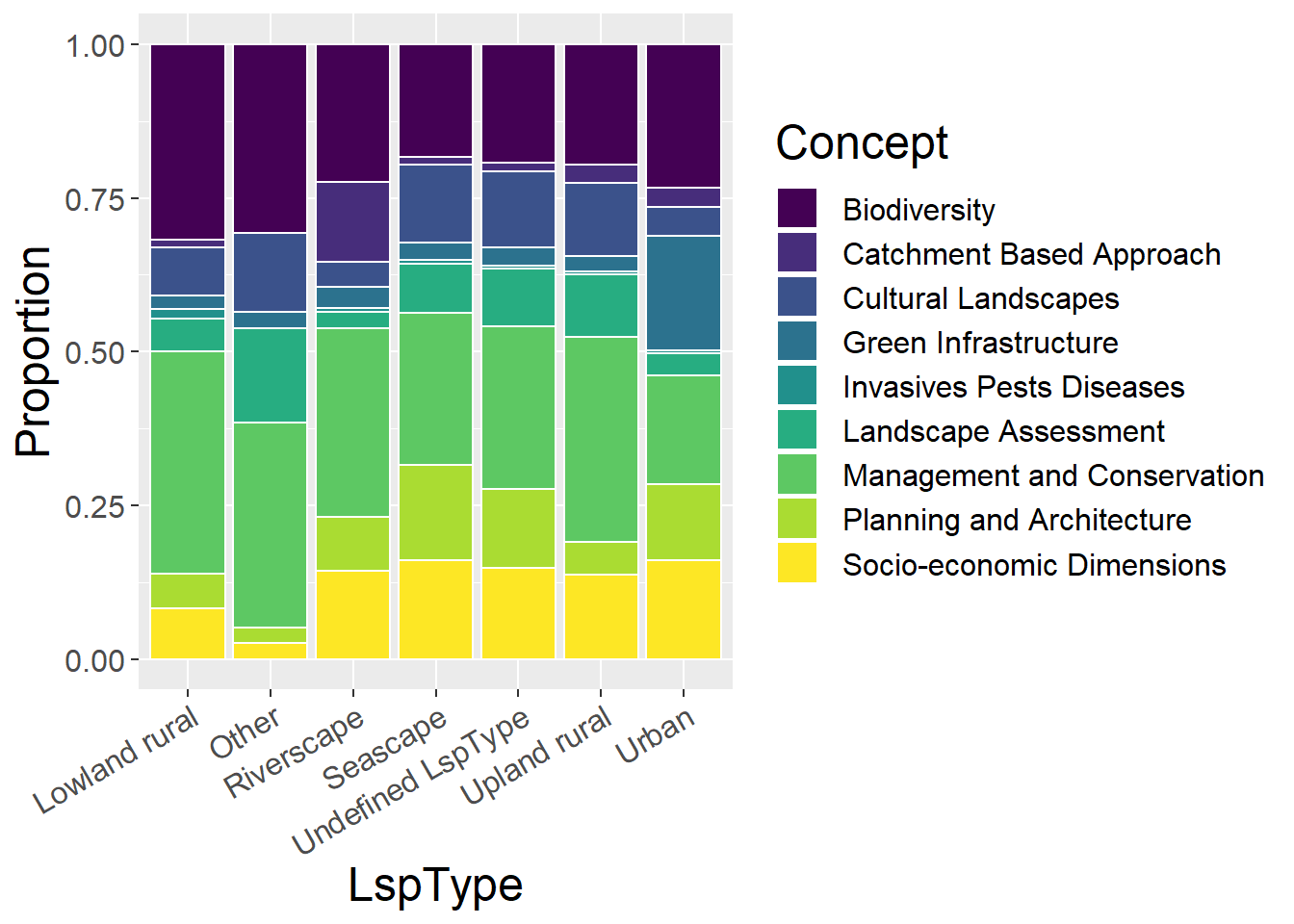
4.8 Other Concepts

General observations:

• Socio-economic dimensions are most widely examined in Urban landscapes and Seascapes
• Unsurprisingly, Green Infrastructure has greatest proportion in Urban landscapes and catchment-based approaches in Riverscapes
• Little study of cultural landscapes in Urban areas

othCCounts <- lspdata %>%
  select(`LspType`,`Green Infrastructure`,`Planning and Architecture`,`Management and Conservation`,`Cultural Landscapes`,`Socio-economic Dimensions`,Biodiversity,`Landscape Assessment`,`Catchment Based Approach`,`Invasives Pests Diseases`) %>%
  mutate(sum = rowSums(.[2:10])) %>%   #calculate total for subsquent calcultation of proportion
  gather(key = Type, value = count, -`LspType`, -sum) %>%
  mutate(prop = count / sum)  #calculate proportion

ggplot(othCCounts, aes(x=`LspType`, y=count, fill=Type)) + geom_bar(stat="identity", colour="white") +
  scale_fill_viridis(discrete = TRUE) +
  theme(axis.text.x = element_text(angle = 30, hjust = 1)) +
  labs(fill="Concept", y = "Abstract Count")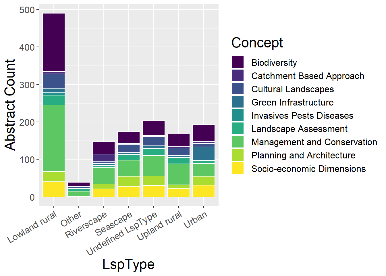

ggplot(othCCounts, aes(x=`LspType`, y=prop, fill=Type)) + geom_bar(stat="identity", colour="white") +
  scale_fill_viridis(discrete = TRUE) +
  theme(axis.text.x = element_text(angle = 30, hjust = 1)) +
  labs(fill="Concept", y = "Proportion")