Chapter 7 Analysis by Spatial Extent

Bar charts and tables to examine how contributions to conferences vary by methods

#spec(cpdata)

spatdata <- cpdata %>%
  select_if(is.numeric) %>%
  gather(key = Spatial, value = count, Micro:`Undefined Extent`) %>%
  filter(count > 0) %>%
  group_by(`Spatial`) %>%
  summarise_all(sum, na.rm=T) 

factor_order <- c('Micro', 'Mini', 'Local', 'Regional', 'National', 'Continental', 'Global','Undefined Extent')
factor_labels <- c('Micro', 'Mini', 'Local', 'Regional', 'National', 'Continental', 'Global','Undefined')

spatdata <- spatdata %>%
  mutate(Spatial = factor(Spatial, levels = factor_order)) %>%
  arrange(Spatial)


uspatdata <- cpdata %>%
  select_if(is.numeric) %>%
  gather(key = Spatial, value = count, Micro:Global) %>%
  filter(count > 0) %>%
  group_by(`Spatial`) %>%
  summarise_all(sum, na.rm=T) 

ufactor_order <- c('Micro', 'Mini', 'Local', 'Regional', 'National', 'Continental', 'Global','Undefined Extent')
ufactor_labels <- c('Micro', 'Mini', 'Local', 'Regional', 'National', 'Continental', 'Global','Undefined')

uspatdata <- uspatdata %>%
  mutate(Spatial = factor(Spatial, levels = ufactor_order)) %>%
  arrange(Spatial)

7.1 Total Conference Contributions

General observations:

• Dominated by Local extent studies, but also many at national and regional extents
• Global and Continental (largest extent) have fewest studies (8 and 27 respectively)

#ggplot(authCounts, aes(x=Spatial, y=count)) + geom_bar(stat="identity")

spatdata %>%
  select(Spatial, count) %>%
  mutate(prop = count/sum(count)) %>%
  mutate(prop = round(prop,3)) %>% 
  kable() %>%
  kable_styling() %>%
  scroll_box(width = "100%")

Spatial	count	prop
Micro	36	0.043
Mini	101	0.120
Local	235	0.278
Regional	172	0.204
National	147	0.174
Continental	29	0.034
Global	9	0.011
Undefined Extent	115	0.136

ggplot(spatdata, aes(x=Spatial, y=count)) + 
  geom_bar(stat="identity") + 
  geom_text(aes(x=Spatial, y=max(count), label = paste0(round(100*count / sum(count),1), "%"), vjust=-0.5))+ theme(axis.text.x = element_text(angle = 15, hjust = 1)) +
  labs(y = "Abstract Count")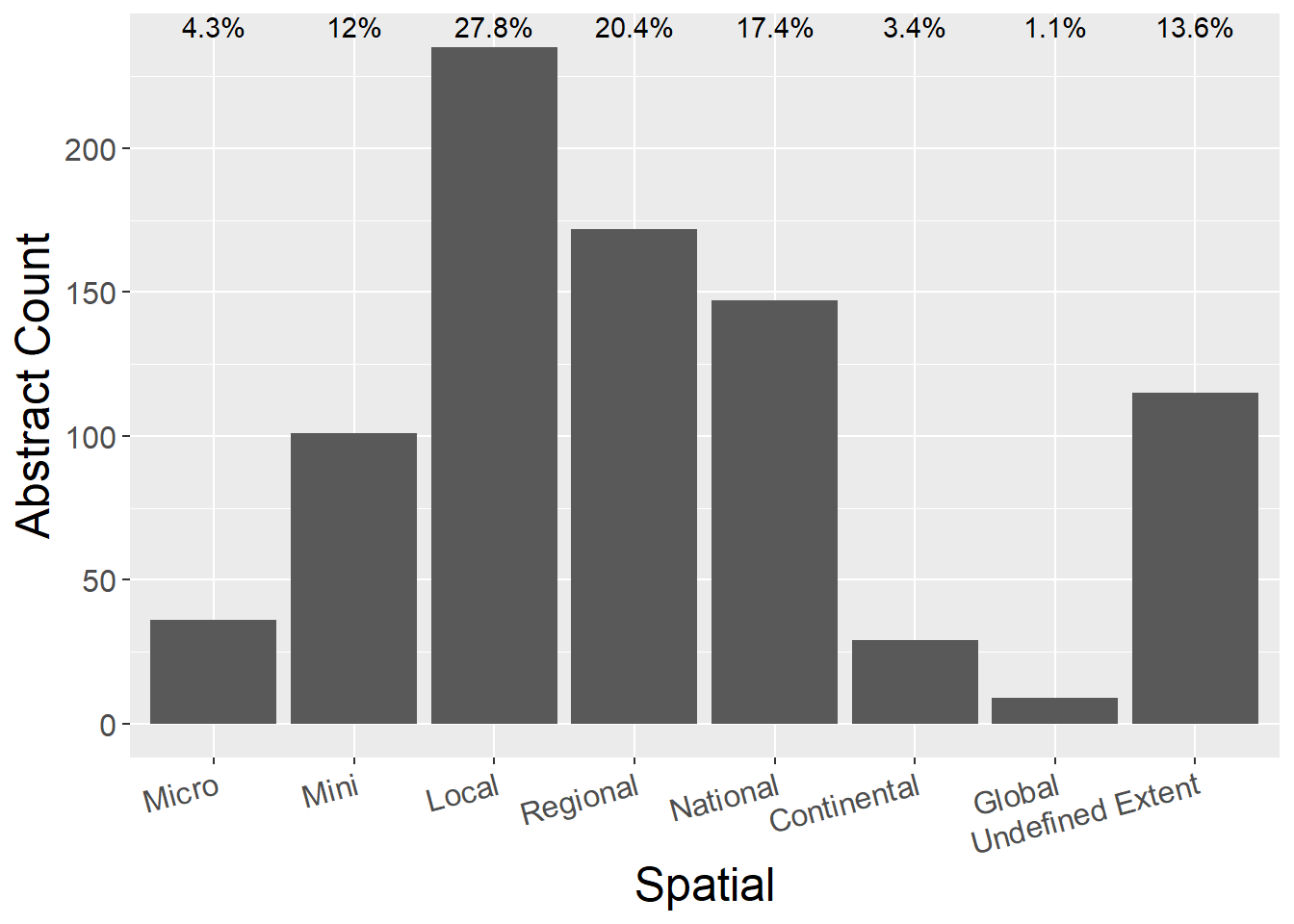

uspatdata %>%
  select(Spatial, count) %>%
  mutate(prop = count/sum(count)) %>%
  mutate(prop = round(prop,3)) %>% 
  kable() %>%
  kable_styling() %>%
  scroll_box(width = "100%")

Spatial	count	prop
Micro	36	0.049
Mini	101	0.139
Local	235	0.322
Regional	172	0.236
National	147	0.202
Continental	29	0.040
Global	9	0.012

ggplot(uspatdata, aes(x=Spatial, y=count)) + 
  geom_bar(stat="identity") + 
  geom_text(aes(x=Spatial, y=max(count), label = paste0(round(100*count / sum(count),1), "%"), vjust=-0.5))+ theme(axis.text.x = element_text(angle = 15, hjust = 1)) +
  labs(y = "Abstract Count")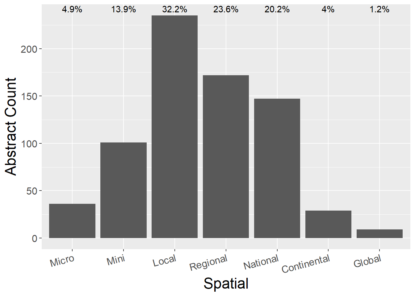

7.2 Author Affiliation

General observations:

• Global studies are have greater proportions of Business and NGO authorship
• All extents dominated by academic authors, except Global and National
• All authorships represented at all extents except Private (in Micro and Global) and Government (in Global)

authCounts <- spatdata %>%
  select(Spatial,Academic, Government,NGO,Business,Private) %>%
  mutate(sum = rowSums(.[2:6])) %>%   #calculate total for subsquent calcultation of proportion
  gather(key = Type, value = count, -Spatial, -sum) %>%
  mutate(prop = count / sum)  #calculate proportion

spatdata %>%
  select(Spatial,Academic, Government,NGO,Business,Private) %>%
  mutate(Total = rowSums(.[2:6])) %>%   #calculate total
  mutate_if(is.numeric, funs(prop = ./ Total)) %>%
  mutate_at(vars(ends_with("prop")), round, 3) %>% 
  select(-Total_prop) %>%
  kable() %>%
  kable_styling() %>%
  scroll_box(width = "100%")

Spatial	Academic	Government	NGO	Business	Private	Total	Academic_prop	Government_prop	NGO_prop	Business_prop	Private_prop
Micro	27	10	3	1	0	41	0.659	0.244	0.073	0.024	0.000
Mini	66	32	12	4	3	117	0.564	0.274	0.103	0.034	0.026
Local	153	71	39	7	8	278	0.550	0.255	0.140	0.025	0.029
Regional	116	49	20	7	2	194	0.598	0.253	0.103	0.036	0.010
National	80	58	18	13	2	171	0.468	0.339	0.105	0.076	0.012
Continental	17	12	1	1	1	32	0.531	0.375	0.031	0.031	0.031
Global	4	0	2	3	0	9	0.444	0.000	0.222	0.333	0.000
Undefined Extent	75	29	13	8	3	128	0.586	0.227	0.102	0.062	0.023

ggplot(authCounts, aes(x=Spatial, y=count, fill=Type)) + geom_bar(stat="identity", colour="white")  +
  scale_fill_viridis(discrete = TRUE) +
  theme(axis.text.x = element_text(angle = 30, hjust = 1)) +
  labs(fill="Affiliation", y = "Abstract Count", x="Extent")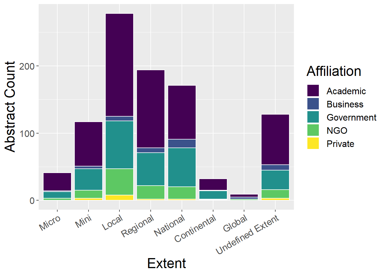

ggplot(authCounts, aes(x=Spatial, y=prop, fill=Type)) + geom_bar(stat="identity", colour="white")  +
  scale_fill_viridis(discrete = TRUE) +
  theme(axis.text.x = element_text(angle = 30, hjust = 1)) +
  labs(fill="Affiliation", y = "Proportion", x="Extent")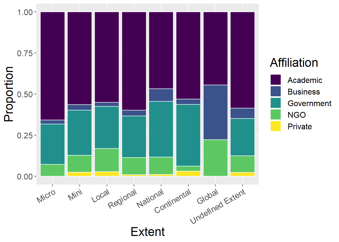

7.3 Landscape Type

7.3.1 Using all landscape types

General observations:

• Global extent studies do not consider Lowland rural landscapes

lspCounts <- spatdata %>%
  select(Spatial,`Upland rural`, `Lowland rural`, Urban,    Riverscape, Seascape, `Undefined LspType`,Other) %>%
  mutate(sum = rowSums(.[2:8])) %>%   #calculate total for subsquent calcultation of proportion
  gather(key = Type, value = count, -Spatial, -sum) %>%
  mutate(prop = count / sum)  #calculate proportion

spatdata %>%
  select(Spatial,`Upland rural`, `Lowland rural`, Urban,    Riverscape, Seascape, `Undefined LspType`,Other) %>%
  mutate(Total = rowSums(.[2:8])) %>%   #calculate total
  mutate_if(is.numeric, funs(prop = ./ Total)) %>%
  mutate_at(vars(ends_with("prop")), round, 3) %>% 
  select(-Total_prop) %>%
  kable() %>%
  kable_styling() %>%
  scroll_box(width = "100%")

Spatial	Upland rural	Lowland rural	Urban	Riverscape	Seascape	Undefined LspType	Other	Total	Upland rural_prop	Lowland rural_prop	Urban_prop	Riverscape_prop	Seascape_prop	Undefined LspType_prop	Other_prop
Micro	4	20	5	4	1	3	1	38	0.105	0.526	0.132	0.105	0.026	0.079	0.026
Mini	14	64	13	15	5	4	1	116	0.121	0.552	0.112	0.129	0.043	0.034	0.009
Local	39	120	47	34	26	15	3	284	0.137	0.423	0.165	0.120	0.092	0.053	0.011
Regional	34	96	14	17	18	9	5	193	0.176	0.497	0.073	0.088	0.093	0.047	0.026
National	36	50	9	14	14	39	11	173	0.208	0.289	0.052	0.081	0.081	0.225	0.064
Continental	4	10	2	4	2	13	5	40	0.100	0.250	0.050	0.100	0.050	0.325	0.125
Global	0	0	2	1	3	4	0	10	0.000	0.000	0.200	0.100	0.300	0.400	0.000
Undefined Extent	4	24	5	18	8	58	4	121	0.033	0.198	0.041	0.149	0.066	0.479	0.033

ggplot(lspCounts, aes(x=Spatial, y=count, fill=Type)) + geom_bar(stat="identity", colour="white")  +
  scale_fill_viridis(discrete = TRUE) +
  theme(axis.text.x = element_text(angle = 30, hjust = 1)) +
  labs(fill="Landscape", y = "Abstract Count", x="Extent")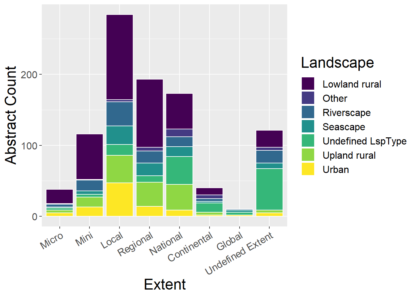

ggplot(lspCounts, aes(x=Spatial, y=prop, fill=Type)) + geom_bar(stat="identity", colour="white")  +
  scale_fill_viridis(discrete = TRUE) +
  theme(axis.text.x = element_text(angle = 30, hjust = 1)) +
  labs(fill="Landscape", y = "Proportion", x="Extent")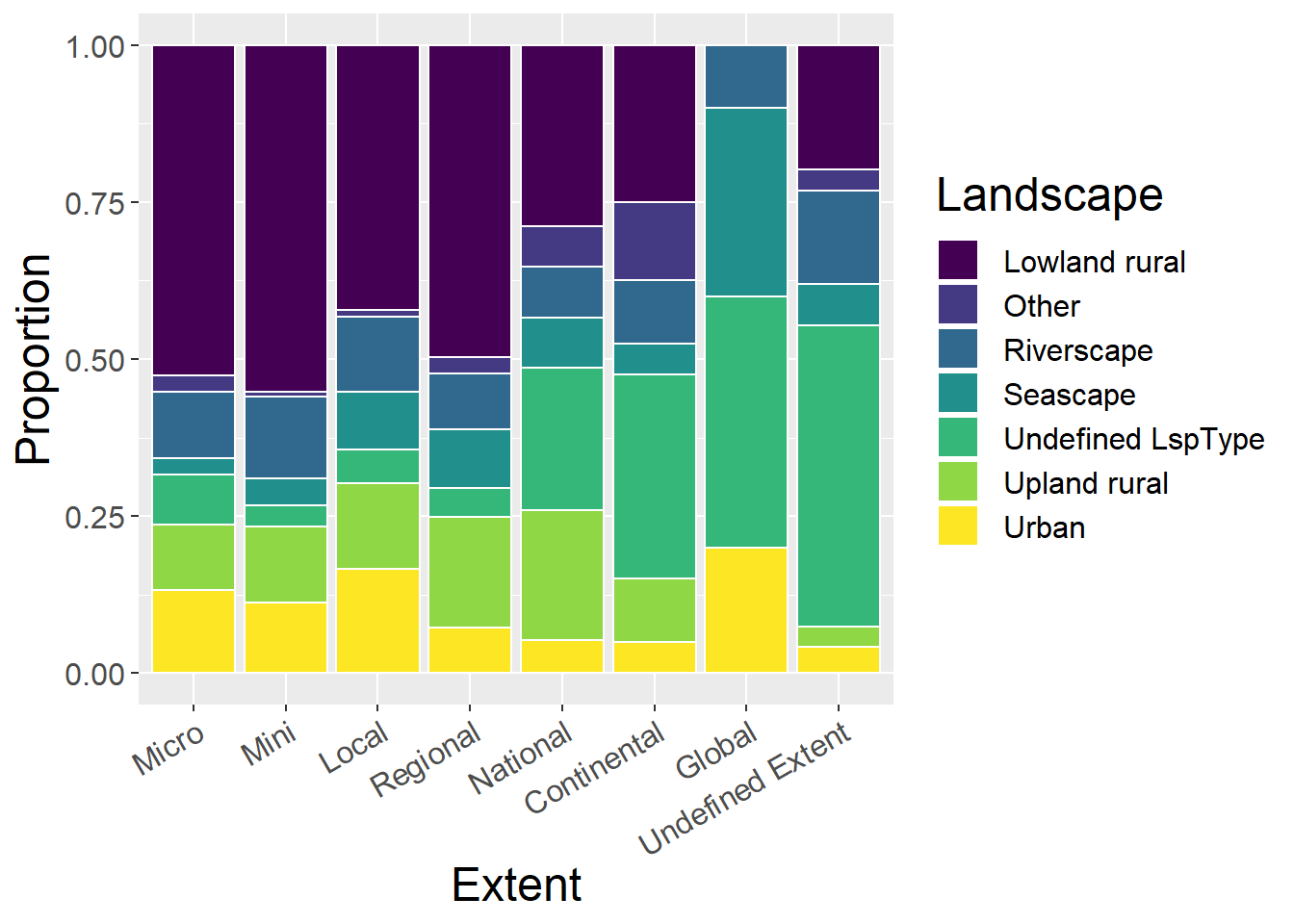

7.3.2 Without ‘Undefined LspType’ and ‘Other’ landscape types

General observations:

• National extent studies have largest proportion of Upland Rural landscape studies
• Micro, Mini and Regional extent studies dominated by Lowland rural
• ‘Undefined extent’ has largest proportion of riverscape studies

lspCounts <- spatdata %>%
  select(Spatial,`Upland rural`, `Lowland rural`, Urban,    Riverscape, Seascape) %>%
  mutate(sum = rowSums(.[2:6])) %>%   #calculate total for subsquent calcultation of proportion
  gather(key = Type, value = count, -Spatial, -sum) %>%
  mutate(prop = count / sum)  #calculate proportion

spatdata %>%
  select(Spatial,`Upland rural`, `Lowland rural`, Urban,    Riverscape, Seascape) %>%
  mutate(Total = rowSums(.[2:6])) %>%   #calculate total
  mutate_if(is.numeric, funs(prop = ./ Total)) %>%
  mutate_at(vars(ends_with("prop")), round, 3) %>% 
  select(-Total_prop) %>%
  kable() %>%
  kable_styling() %>%
  scroll_box(width = "100%")

Spatial	Upland rural	Lowland rural	Urban	Riverscape	Seascape	Total	Upland rural_prop	Lowland rural_prop	Urban_prop	Riverscape_prop	Seascape_prop
Micro	4	20	5	4	1	34	0.118	0.588	0.147	0.118	0.029
Mini	14	64	13	15	5	111	0.126	0.577	0.117	0.135	0.045
Local	39	120	47	34	26	266	0.147	0.451	0.177	0.128	0.098
Regional	34	96	14	17	18	179	0.190	0.536	0.078	0.095	0.101
National	36	50	9	14	14	123	0.293	0.407	0.073	0.114	0.114
Continental	4	10	2	4	2	22	0.182	0.455	0.091	0.182	0.091
Global	0	0	2	1	3	6	0.000	0.000	0.333	0.167	0.500
Undefined Extent	4	24	5	18	8	59	0.068	0.407	0.085	0.305	0.136

ggplot(lspCounts, aes(x=Spatial, y=count, fill=Type)) + geom_bar(stat="identity", colour="white") +
  scale_fill_viridis(discrete = TRUE) +
  theme(axis.text.x = element_text(angle = 30, hjust = 1)) +
  labs(fill="Landscape", y = "Abstract Count", x="Extent")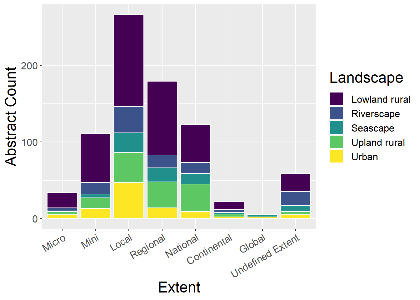

ggplot(lspCounts, aes(x=Spatial, y=prop, fill=Type)) + geom_bar(stat="identity", colour="white") +
  scale_fill_viridis(discrete = TRUE) +
  theme(axis.text.x = element_text(angle = 30, hjust = 1)) +
  labs(fill="Landscape", y = "Proportion", x="Extent")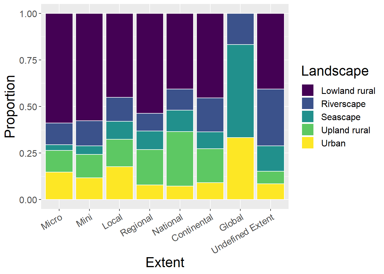

7.4 Organism

General observations:

• Global studies are again qualitatively different from other scale studies - no amphibiams, birds, reptiles, woodland studies but largest proportions of Fish and generic Habitat studies
• Smallest extents (mini and micro) have largest proportions of Plant and Inverts studies

speciesCounts <- spatdata %>%
  select(Spatial, Mammals, Humans, Birds, Reptiles, Inverts, Plants, Amphibians, Fish, `Generic Habitat`,`Woodland Forests`) %>%
  mutate(sum = rowSums(.[2:11])) %>%   #calculate total for subsquent calcultation of proportion
  gather(key = Type, value = count, -Spatial, -sum) %>%
  mutate(prop = count / sum)  #calculate proportion

spatdata %>%
  select(Spatial, Mammals, Humans, Birds, Reptiles, Inverts, Plants, Amphibians, Fish, `Generic Habitat`,`Woodland Forests`) %>%
  mutate(Total = rowSums(.[2:11])) %>%   #calculate total for subsquent calcultation of proportion
  mutate_if(is.numeric, funs(prop = ./ Total)) %>%
  mutate_at(vars(ends_with("prop")), round, 3) %>% 
  select(-Total_prop) %>%
  kable() %>%
  kable_styling() %>%
  scroll_box(width = "100%")

Spatial	Mammals	Humans	Birds	Reptiles	Inverts	Plants	Amphibians	Fish	Generic Habitat	Woodland Forests	Total	Mammals_prop	Humans_prop	Birds_prop	Reptiles_prop	Inverts_prop	Plants_prop	Amphibians_prop	Fish_prop	Generic Habitat_prop	Woodland Forests_prop
Micro	1	0	6	0	18	17	3	0	3	3	51	0.020	0.000	0.118	0.000	0.353	0.333	0.059	0.000	0.059	0.059
Mini	6	5	23	0	39	25	1	3	17	16	135	0.044	0.037	0.170	0.000	0.289	0.185	0.007	0.022	0.126	0.119
Local	15	32	43	2	25	29	5	3	74	53	281	0.053	0.114	0.153	0.007	0.089	0.103	0.018	0.011	0.263	0.189
Regional	7	17	26	2	12	20	2	3	52	40	181	0.039	0.094	0.144	0.011	0.066	0.110	0.011	0.017	0.287	0.221
National	8	19	16	2	10	20	0	0	49	34	158	0.051	0.120	0.101	0.013	0.063	0.127	0.000	0.000	0.310	0.215
Continental	1	6	4	0	1	4	0	0	12	4	32	0.031	0.188	0.125	0.000	0.031	0.125	0.000	0.000	0.375	0.125
Global	0	1	0	0	0	1	0	2	4	0	8	0.000	0.125	0.000	0.000	0.000	0.125	0.000	0.250	0.500	0.000
Undefined Extent	6	11	15	1	10	10	1	1	35	17	107	0.056	0.103	0.140	0.009	0.093	0.093	0.009	0.009	0.327	0.159

ggplot(speciesCounts, aes(x=Spatial, y=count, fill=Type)) + geom_bar(stat="identity", colour="white") +
  scale_fill_viridis(discrete = TRUE) +
  theme(axis.text.x = element_text(angle = 30, hjust = 1)) +
  labs(fill="Organism", y = "Abstract Count", x="Extent")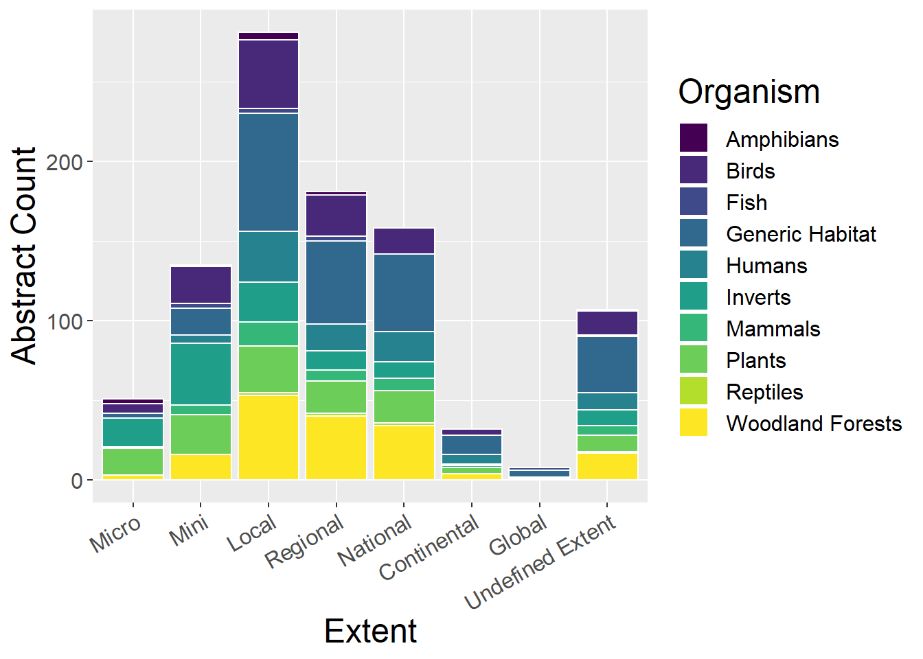

ggplot(speciesCounts, aes(x=Spatial, y=prop, fill=Type)) + geom_bar(stat="identity", colour="white") +
  scale_fill_viridis(discrete = TRUE) +
  theme(axis.text.x = element_text(angle = 30, hjust = 1)) +
  labs(fill="Organism", y = "Proportion", x="Extent")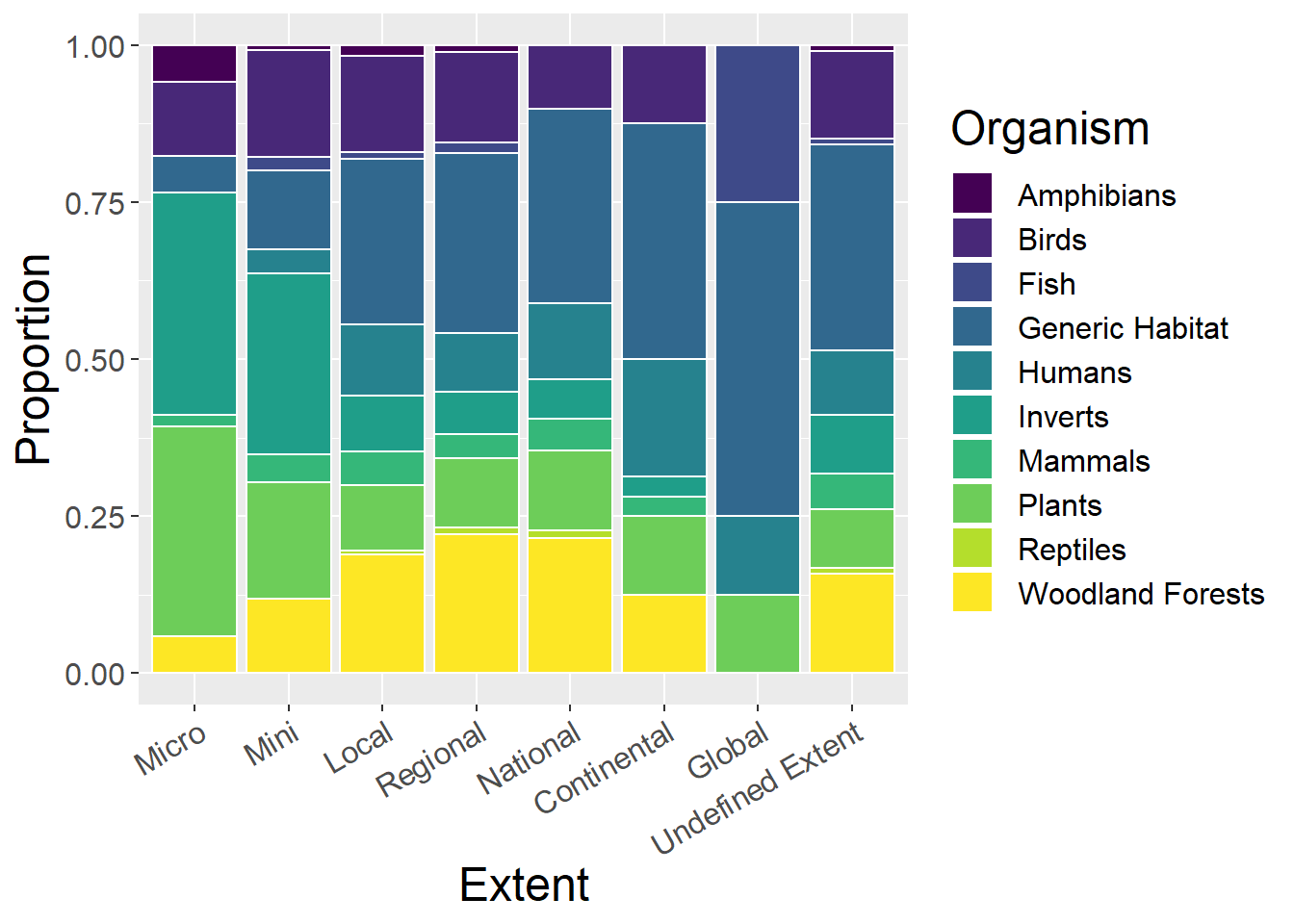

7.5 Methods

General observations:

• Global, Continental and Undefined Extent have the greatest proportions of Theoretical, Qualitative and Remote Sensing studies
• Smallest extents (mini and micro) have the largest proportions of Empirical studies (and local have largest absolute number)
• Regional and Local studies have largest number and proportions of GIS studies (and GIS used least at extremes of extents, i.e. mini, micro and global)

methodsCounts <- spatdata %>%
  select(Spatial, Empirical, Theoretical, Qualitative, Quantitative, GIS, `Remote sensing`) %>%
  mutate(sum = rowSums(.[2:7])) %>%
  gather(key = Type, value = count, -Spatial, -sum) %>%
  mutate(prop = count / sum) 

spatdata %>%
  select(Spatial, Empirical, Theoretical, Qualitative, Quantitative, GIS, `Remote sensing`) %>%
  mutate(Total = rowSums(.[2:7])) %>%
  mutate_if(is.numeric, funs(prop = ./ Total)) %>%
  mutate_at(vars(ends_with("prop")), round, 3) %>% 
  select(-Total_prop) %>%
  kable() %>%
  kable_styling() %>%
  scroll_box(width = "100%")

Spatial	Empirical	Theoretical	Qualitative	Quantitative	GIS	Remote sensing	Total	Empirical_prop	Theoretical_prop	Qualitative_prop	Quantitative_prop	GIS_prop	Remote sensing_prop
Micro	27	4	0	17	4	1	53	0.509	0.075	0.000	0.321	0.075	0.019
Mini	72	9	9	53	13	5	161	0.447	0.056	0.056	0.329	0.081	0.031
Local	115	28	52	102	73	14	384	0.299	0.073	0.135	0.266	0.190	0.036
Regional	82	33	29	93	65	12	314	0.261	0.105	0.092	0.296	0.207	0.038
National	56	44	40	69	35	4	248	0.226	0.177	0.161	0.278	0.141	0.016
Continental	6	11	14	11	9	3	54	0.111	0.204	0.259	0.204	0.167	0.056
Global	2	5	4	4	1	1	17	0.118	0.294	0.235	0.235	0.059	0.059
Undefined Extent	35	56	24	34	11	5	165	0.212	0.339	0.145	0.206	0.067	0.030

ggplot(methodsCounts, aes(x=Spatial, y=count, fill=Type)) + geom_bar(stat="identity", colour="white") +
  scale_fill_viridis(discrete = TRUE) +
  theme(axis.text.x = element_text(angle = 30, hjust = 1)) +
  labs(fill="Method", y = "Abstract Count", x="Extent")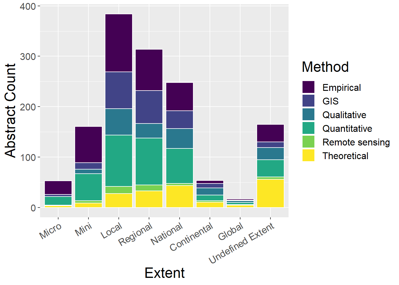

ggplot(methodsCounts, aes(x=Spatial, y=prop, fill=Type)) + geom_bar(stat="identity", colour="white") +
  scale_fill_viridis(discrete = TRUE) +
  theme(axis.text.x = element_text(angle = 30, hjust = 1)) +
  labs(fill="Method", y = "Proportion", x="Extent")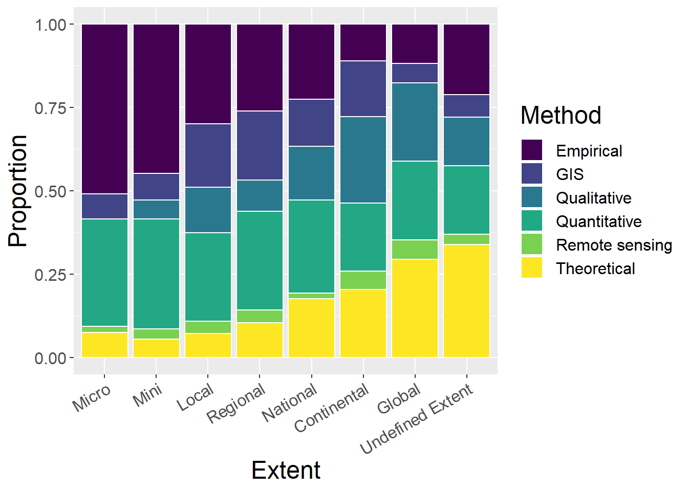

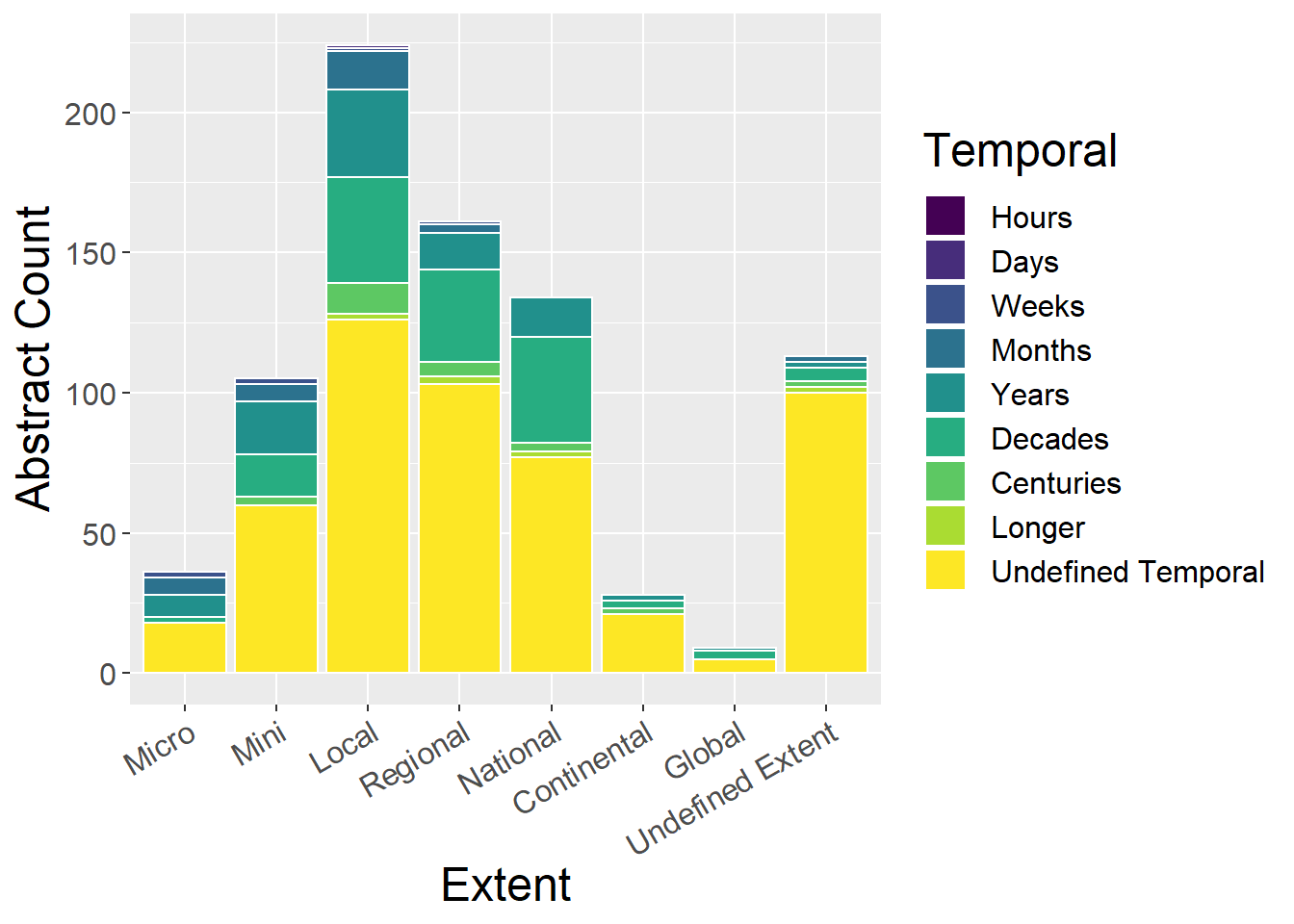
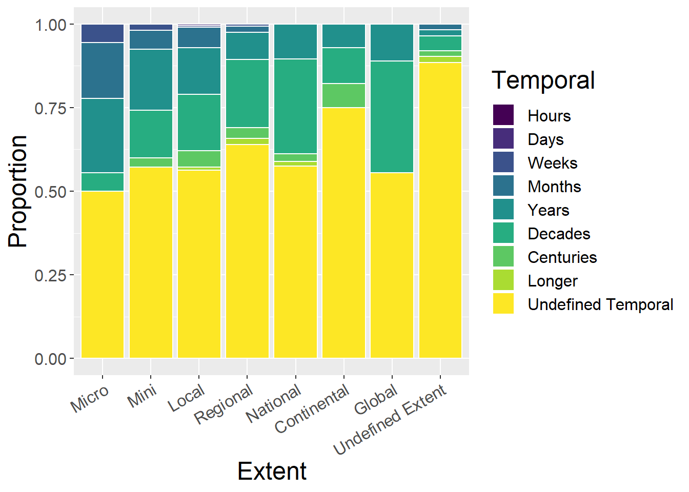
7.6 Temporal Extent

7.6.1 With undefined

General observations:

Spatial	Hours	Days	Weeks	Months	Years	Decades	Centuries	Longer	Undefined Temporal	Total	Hours_prop	Days_prop	Weeks_prop	Months_prop	Years_prop	Decades_prop	Centuries_prop	Longer_prop	Undefined Temporal_prop
Micro	0	0	2	6	8	2	0	0	18	36	0	0.000	0.056	0.167	0.222	0.056	0.000	0.000	0.500
Mini	0	0	2	6	19	15	3	0	60	105	0	0.000	0.019	0.057	0.181	0.143	0.029	0.000	0.571
Local	0	1	1	14	31	38	11	2	126	224	0	0.004	0.004	0.062	0.138	0.170	0.049	0.009	0.562
Regional	0	0	1	3	13	33	5	3	103	161	0	0.000	0.006	0.019	0.081	0.205	0.031	0.019	0.640
National	0	0	0	0	14	38	3	2	77	134	0	0.000	0.000	0.000	0.104	0.284	0.022	0.015	0.575
Continental	0	0	0	0	2	3	2	0	21	28	0	0.000	0.000	0.000	0.071	0.107	0.071	0.000	0.750
Global	0	0	0	0	1	3	0	0	5	9	0	0.000	0.000	0.000	0.111	0.333	0.000	0.000	0.556
Undefined Extent	0	0	0	2	2	5	2	2	100	113	0	0.000	0.000	0.018	0.018	0.044	0.018	0.018	0.885

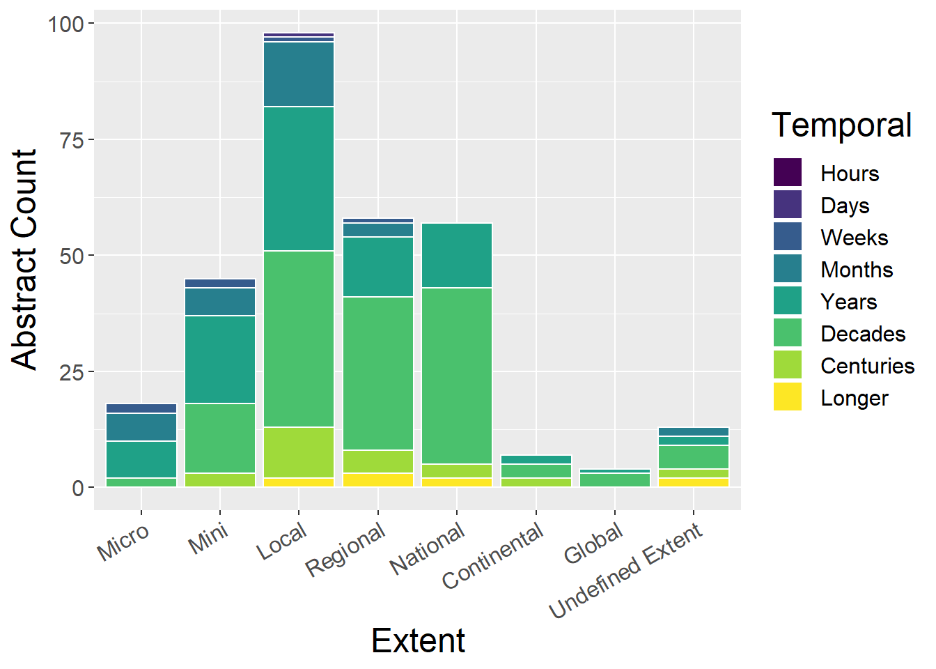
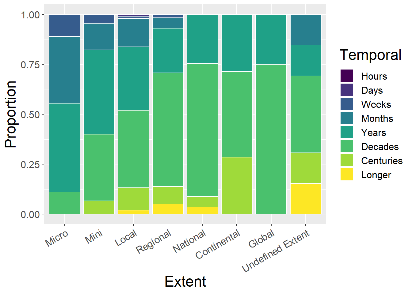
7.6.2 Without Undefined

• Again Global is qualitatively different (only Decades and Years studies)
• Continental has nothing shorter than Years
• National and Regional extents have large proportions of Decadal studies
• Micro and Mini extents have largest proprtions of Monthly and Weekly studies

Spatial	Hours	Days	Weeks	Months	Years	Decades	Centuries	Longer	Total	Hours_prop	Days_prop	Weeks_prop	Months_prop	Years_prop	Decades_prop	Centuries_prop	Longer_prop
Micro	0	0	2	6	8	2	0	0	18	0	0.00	0.111	0.333	0.444	0.111	0.000	0.000
Mini	0	0	2	6	19	15	3	0	45	0	0.00	0.044	0.133	0.422	0.333	0.067	0.000
Local	0	1	1	14	31	38	11	2	98	0	0.01	0.010	0.143	0.316	0.388	0.112	0.020
Regional	0	0	1	3	13	33	5	3	58	0	0.00	0.017	0.052	0.224	0.569	0.086	0.052
National	0	0	0	0	14	38	3	2	57	0	0.00	0.000	0.000	0.246	0.667	0.053	0.035
Continental	0	0	0	0	2	3	2	0	7	0	0.00	0.000	0.000	0.286	0.429	0.286	0.000
Global	0	0	0	0	1	3	0	0	4	0	0.00	0.000	0.000	0.250	0.750	0.000	0.000
Undefined Extent	0	0	0	2	2	5	2	2	13	0	0.00	0.000	0.154	0.154	0.385	0.154	0.154

7.7 Concepts

General observations:

• Global extents have largest proportions of Ecosystem Services and Climate Change studies
• Continental and National extents have largest proportions of LUCC studies
• Micro extent have largest proportion of Pattern-Process-Scale studies

conceptCounts <- spatdata %>%
  select(Spatial, `PPS of landscapes`,
`Connectivity and fragmentation`, `Scale and scaling`,`Spatial analysis and modeling`,LUCC,`History and legacy`,`Climate change interactions`,`Ecosystem services`,`Landscape sustainability`,`Accuracy and uncertainty`
) %>%
  mutate(sum = rowSums(.[2:11])) %>%
  gather(key = Type, value = count, -Spatial, -sum) %>%
  mutate(prop = count / sum) 


spatdata %>%
  select(Spatial, `PPS of landscapes`,
`Connectivity and fragmentation`, `Scale and scaling`,`Spatial analysis and modeling`,LUCC,`History and legacy`,`Climate change interactions`,`Ecosystem services`,`Landscape sustainability`,`Accuracy and uncertainty`
) %>%
  mutate(Total = rowSums(.[2:11])) %>%
  mutate_if(is.numeric, funs(prop = ./ Total)) %>%
  mutate_at(vars(ends_with("prop")), round, 3) %>% 
  select(-Total_prop) %>%
  kable() %>%
  kable_styling() %>%
  scroll_box(width = "100%")

Spatial	PPS of landscapes	Connectivity and fragmentation	Scale and scaling	Spatial analysis and modeling	LUCC	History and legacy	Climate change interactions	Ecosystem services	Landscape sustainability	Accuracy and uncertainty	Total	PPS of landscapes_prop	Connectivity and fragmentation_prop	Scale and scaling_prop	Spatial analysis and modeling_prop	LUCC_prop	History and legacy_prop	Climate change interactions_prop	Ecosystem services_prop	Landscape sustainability_prop	Accuracy and uncertainty_prop
Micro	11	7	6	7	7	0	0	1	0	0	39	0.282	0.179	0.154	0.179	0.179	0.000	0.000	0.026	0.000	0.000
Mini	20	25	12	16	20	8	4	6	7	1	119	0.168	0.210	0.101	0.134	0.168	0.067	0.034	0.050	0.059	0.008
Local	33	71	18	67	73	25	15	33	27	2	364	0.091	0.195	0.049	0.184	0.201	0.069	0.041	0.091	0.074	0.005
Regional	19	48	10	58	62	30	15	22	27	1	292	0.065	0.164	0.034	0.199	0.212	0.103	0.051	0.075	0.092	0.003
National	12	25	8	31	59	22	8	25	21	2	213	0.056	0.117	0.038	0.146	0.277	0.103	0.038	0.117	0.099	0.009
Continental	1	4	2	7	13	5	1	5	6	0	44	0.023	0.091	0.045	0.159	0.295	0.114	0.023	0.114	0.136	0.000
Global	2	2	1	1	3	2	2	6	2	0	21	0.095	0.095	0.048	0.048	0.143	0.095	0.095	0.286	0.095	0.000
Undefined Extent	16	30	9	21	15	5	5	22	13	1	137	0.117	0.219	0.066	0.153	0.109	0.036	0.036	0.161	0.095	0.007

ggplot(conceptCounts, aes(x=Spatial, y=count, fill=Type)) + geom_bar(stat="identity", colour="white") +
  scale_fill_viridis(discrete = TRUE) +
  theme(axis.text.x = element_text(angle = 30, hjust = 1)) +
  labs(fill="Concept", y = "Abstract Count", x="Extent")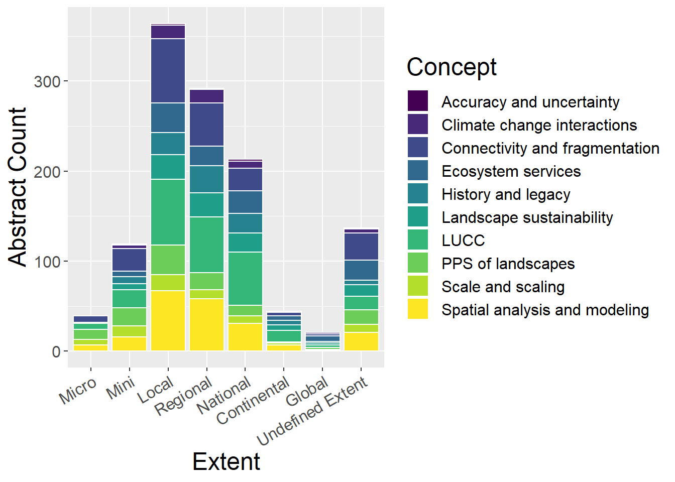

ggplot(conceptCounts, aes(x=Spatial, y=prop, fill=Type)) + geom_bar(stat="identity", colour="white") +
  scale_fill_viridis(discrete = TRUE) +
  theme(axis.text.x = element_text(angle = 30, hjust = 1)) +
  labs(fill="Concept", y = "Proportion", x="Extent")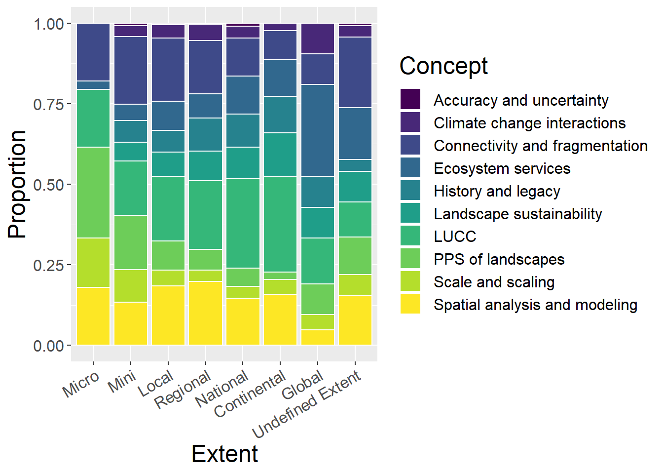

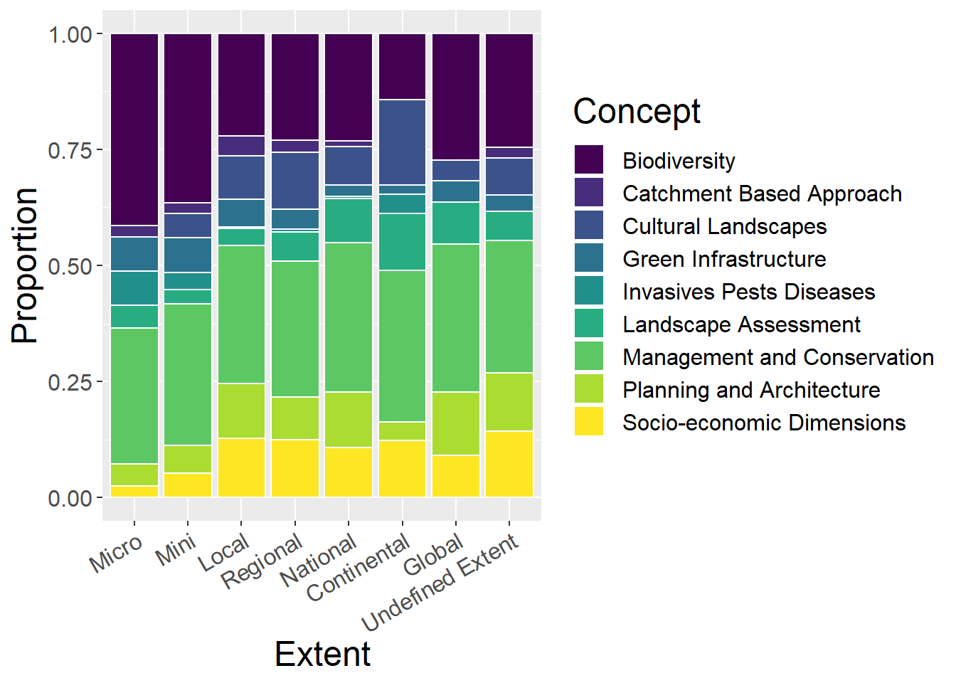
7.8 Other Concepts

General observations:

• Smallest extents (micro and mini) have smallest proportions of Socio-Economic Dimensions studies and largest proportions of Biodiversity studies
• Consistent proportions of Management and Conservation studies across all extents

otherCounts <- spatdata %>%
  select(Spatial, `Green Infrastructure`,`Planning and Architecture`,`Management and Conservation`,`Cultural Landscapes`,`Socio-economic Dimensions`,Biodiversity,`Landscape Assessment`,`Catchment Based Approach`,`Invasives Pests Diseases`
) %>%
  mutate(sum = rowSums(.[2:10])) %>%
  gather(key = Type, value = count, -Spatial, -sum) %>%
  mutate(prop = count / sum) 

spatdata %>%
  select(Spatial, `Green Infrastructure`,`Planning and Architecture`,`Management and Conservation`,`Cultural Landscapes`,`Socio-economic Dimensions`,Biodiversity,`Landscape Assessment`,`Catchment Based Approach`,`Invasives Pests Diseases`
) %>%
  mutate(Total = rowSums(.[2:10])) %>%
  mutate_if(is.numeric, funs(prop = ./ Total)) %>%
  mutate_at(vars(ends_with("prop")), round, 3) %>% 
  select(-Total_prop) %>%
  kable() %>%
  kable_styling() %>%
  scroll_box(width = "100%")

Spatial	Green Infrastructure	Planning and Architecture	Management and Conservation	Cultural Landscapes	Socio-economic Dimensions	Biodiversity	Landscape Assessment	Catchment Based Approach	Invasives Pests Diseases	Total	Green Infrastructure_prop	Planning and Architecture_prop	Management and Conservation_prop	Cultural Landscapes_prop	Socio-economic Dimensions_prop	Biodiversity_prop	Landscape Assessment_prop	Catchment Based Approach_prop	Invasives Pests Diseases_prop
Micro	3	2	12	0	1	17	2	1	3	41	0.073	0.049	0.293	0.000	0.024	0.415	0.049	0.024	0.073
Mini	10	8	41	7	7	49	4	3	5	134	0.075	0.060	0.306	0.052	0.052	0.366	0.030	0.022	0.037
Local	22	43	109	34	47	81	14	16	1	367	0.060	0.117	0.297	0.093	0.128	0.221	0.038	0.044	0.003
Regional	13	28	89	37	38	70	19	8	2	304	0.043	0.092	0.293	0.122	0.125	0.230	0.062	0.026	0.007
National	6	28	75	19	25	54	22	3	1	233	0.026	0.120	0.322	0.082	0.107	0.232	0.094	0.013	0.004
Continental	1	2	16	9	6	7	6	0	2	49	0.020	0.041	0.327	0.184	0.122	0.143	0.122	0.000	0.041
Global	1	3	7	1	2	6	2	0	0	22	0.045	0.136	0.318	0.045	0.091	0.273	0.091	0.000	0.000
Undefined Extent	6	22	50	14	25	43	11	4	0	175	0.034	0.126	0.286	0.080	0.143	0.246	0.063	0.023	0.000

ggplot(otherCounts, aes(x=Spatial, y=count, fill=Type)) + geom_bar(stat="identity", colour="white")+
  scale_fill_viridis(discrete = TRUE) +
  theme(axis.text.x = element_text(angle = 30, hjust = 1)) +
  labs(fill="Concept", y = "Abstract Count", x="Extent")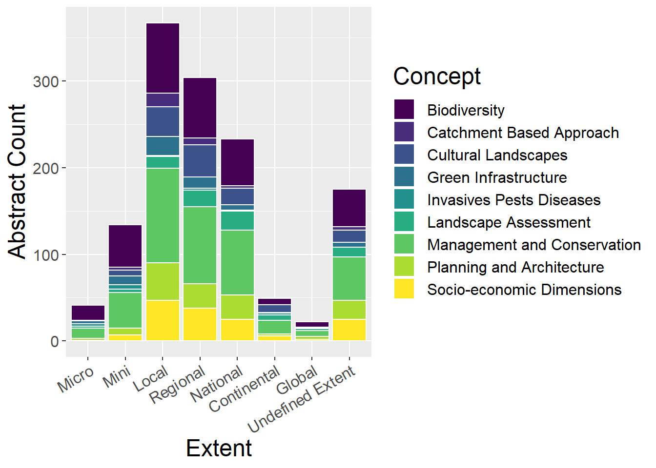

ggplot(otherCounts, aes(x=Spatial, y=prop, fill=Type)) + geom_bar(stat="identity", colour="white")+
  scale_fill_viridis(discrete = TRUE) +
  theme(axis.text.x = element_text(angle = 30, hjust = 1)) +
  labs(fill="Concept", y = "Proportion", x="Extent")