Chapter 9 Analysis by Concept | 25 years of ialeUK conferences: An analysis

9.1 Total Conference Contributions

General observations:

Connectivity & fragmentation, LUCC and spatial analysis & modelling most frequent (composing > 50%)

#ggplot(authCounts, aes(x=Concept, y=count)) + geom_bar(stat="identity")

conceptdata %>%
  select(Concept, count) %>%
  mutate(prop = count/sum(count)) %>%
  mutate(prop = round(prop,3)) %>% 
  kable() %>%
  kable_styling() %>%
  scroll_box(width = "100%")

Concept	count	prop
Accuracy and uncertainty	6	0.005
Climate change interactions	45	0.040
Connectivity and fragmentation	205	0.184
Ecosystem services	108	0.097
History and legacy	89	0.080
Landscape sustainability	98	0.088
LUCC	224	0.201
PPS of landscapes	105	0.094
Scale and scaling	54	0.049
Spatial analysis and modeling	179	0.161

ggplot(conceptdata, aes(x=Concept, y=count)) + 
  geom_bar(stat="identity") + 
  geom_text(aes(x=Concept, y=max(count), label = paste0(round(100*count / sum(count),1), "%"), vjust=-0.25)) + 
  theme(axis.text.x = element_text(angle = 45, hjust = 1))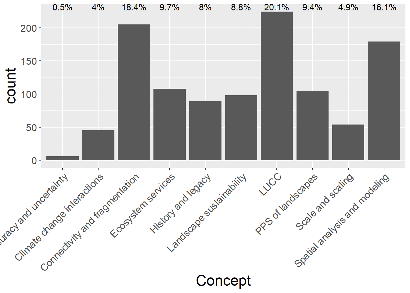

9.2 Author Affiliation

General observations:

No obvious differences between concepts

authCounts <- conceptdata %>%
  select(Concept,Academic, Government,NGO,Business,Private) %>%
  mutate(sum = rowSums(.[2:6])) %>%   #calculate total for subsquent calcultation of proportion
  gather(key = Type, value = count, -Concept, -sum) %>%
  mutate(prop = count / sum)  #calculate proportion

conceptdata %>%
  select(Concept,Academic, Government,NGO,Business,Private) %>%
  mutate(Total = rowSums(.[2:6])) %>%   #calculate total
  mutate_if(is.numeric, funs(prop = ./ Total)) %>%
  mutate_at(vars(ends_with("prop")), round, 3) %>% 
  select(-Total_prop) %>%
  kable() %>%
  kable_styling() %>%
  scroll_box(width = "100%")

Concept	Academic	Government	NGO	Business	Private	Total	Academic_prop	Government_prop	NGO_prop	Business_prop	Private_prop
Accuracy and uncertainty	4	3	1	0	1	9	0.444	0.333	0.111	0.000	0.111
Climate change interactions	28	7	10	5	0	50	0.560	0.140	0.200	0.100	0.000
Connectivity and fragmentation	129	72	21	8	3	233	0.554	0.309	0.090	0.034	0.013
Ecosystem services	65	18	19	12	3	117	0.556	0.154	0.162	0.103	0.026
History and legacy	56	24	14	1	1	96	0.583	0.250	0.146	0.010	0.010
Landscape sustainability	52	30	17	6	3	108	0.481	0.278	0.157	0.056	0.028
LUCC	150	64	27	9	1	251	0.598	0.255	0.108	0.036	0.004
PPS of landscapes	74	36	9	1	0	120	0.617	0.300	0.075	0.008	0.000
Scale and scaling	36	17	5	1	0	59	0.610	0.288	0.085	0.017	0.000
Spatial analysis and modeling	122	55	19	10	3	209	0.584	0.263	0.091	0.048	0.014

ggplot(authCounts, aes(x=Concept, y=count, fill=Type)) + 
  geom_bar(stat="identity", colour="white") + 
  theme(axis.text.x = element_text(angle = 45, hjust = 1)) +
  scale_fill_viridis(discrete = TRUE) +
  labs(fill="Affiliation", y = "Abstract Count", x="Concept")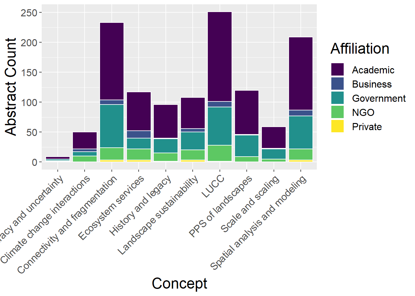

ggplot(authCounts, aes(x=Concept, y=prop, fill=Type)) + 
  geom_bar(stat="identity", colour="white") + 
  theme(axis.text.x = element_text(angle = 45, hjust = 1)) +
  scale_fill_viridis(discrete = TRUE) +
  labs(fill="Affiliation", y = "Proportion", x="Concept")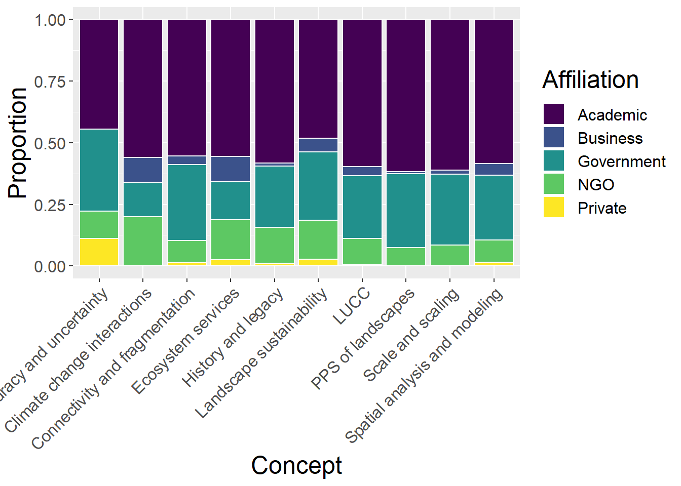

9.3 Landscape Type

9.3.1 Using all landscape types

General observations:

Ecosystem services have greatest proportion of urban landscapes and lowest in lowland rural
Connectivity & Fragmentation have greatest proportion of studies in Lowland rural landscapes

lspCounts <- conceptdata %>%
  select(Concept,`Upland rural`, `Lowland rural`, Urban,    Riverscape, Seascape, `Undefined LspType`,Other) %>%
  mutate(sum = rowSums(.[2:8])) %>%   #calculate total for subsquent calcultation of proportion
  gather(key = Type, value = count, -Concept, -sum) %>%
  mutate(prop = count / sum)  #calculate proportion

conceptdata %>%
  select(Concept,`Upland rural`, `Lowland rural`, Urban,    Riverscape, Seascape, `Undefined LspType`,Other) %>%
  mutate(Total = rowSums(.[2:8])) %>%   #calculate total
  mutate_if(is.numeric, funs(prop = ./ Total)) %>%
  mutate_at(vars(ends_with("prop")), round, 3) %>% 
  select(-Total_prop) %>%
  kable() %>%
  kable_styling() %>%
  scroll_box(width = "100%")

Concept	Upland rural	Lowland rural	Urban	Riverscape	Seascape	Undefined LspType	Other	Total	Upland rural_prop	Lowland rural_prop	Urban_prop	Riverscape_prop	Seascape_prop	Undefined LspType_prop	Other_prop
Accuracy and uncertainty	1	0	0	3	0	3	0	7	0.143	0.000	0.000	0.429	0.000	0.429	0.000
Climate change interactions	9	12	12	8	11	6	0	58	0.155	0.207	0.207	0.138	0.190	0.103	0.000
Connectivity and fragmentation	16	112	24	15	12	31	7	217	0.074	0.516	0.111	0.069	0.055	0.143	0.032
Ecosystem services	15	24	27	12	20	24	1	123	0.122	0.195	0.220	0.098	0.163	0.195	0.008
History and legacy	18	47	3	16	9	14	4	111	0.162	0.423	0.027	0.144	0.081	0.126	0.036
Landscape sustainability	19	41	10	9	17	22	2	120	0.158	0.342	0.083	0.075	0.142	0.183	0.017
LUCC	56	109	22	32	14	31	8	272	0.206	0.401	0.081	0.118	0.051	0.114	0.029
PPS of landscapes	15	45	13	17	7	15	3	115	0.130	0.391	0.113	0.148	0.061	0.130	0.026
Scale and scaling	10	21	8	8	6	9	4	66	0.152	0.318	0.121	0.121	0.091	0.136	0.061
Spatial analysis and modeling	22	88	22	19	14	25	4	194	0.113	0.454	0.113	0.098	0.072	0.129	0.021

ggplot(lspCounts, aes(x=Concept, y=count, fill=Type)) + 
  geom_bar(stat="identity", colour="white") + 
  theme(axis.text.x = element_text(angle = 45, hjust = 1)) +
  scale_fill_viridis(discrete = TRUE) +
  labs(fill="Landscape", y = "Abstract Count", x="Concept")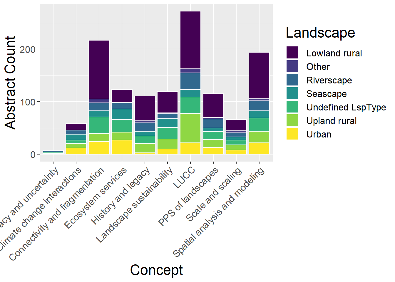

ggplot(lspCounts, aes(x=Concept, y=prop, fill=Type)) + 
  geom_bar(stat="identity", colour="white") + 
  theme(axis.text.x = element_text(angle = 45, hjust = 1)) +
  scale_fill_viridis(discrete = TRUE) +
  labs(fill="Landscape", y = "Proportion", x="Concept")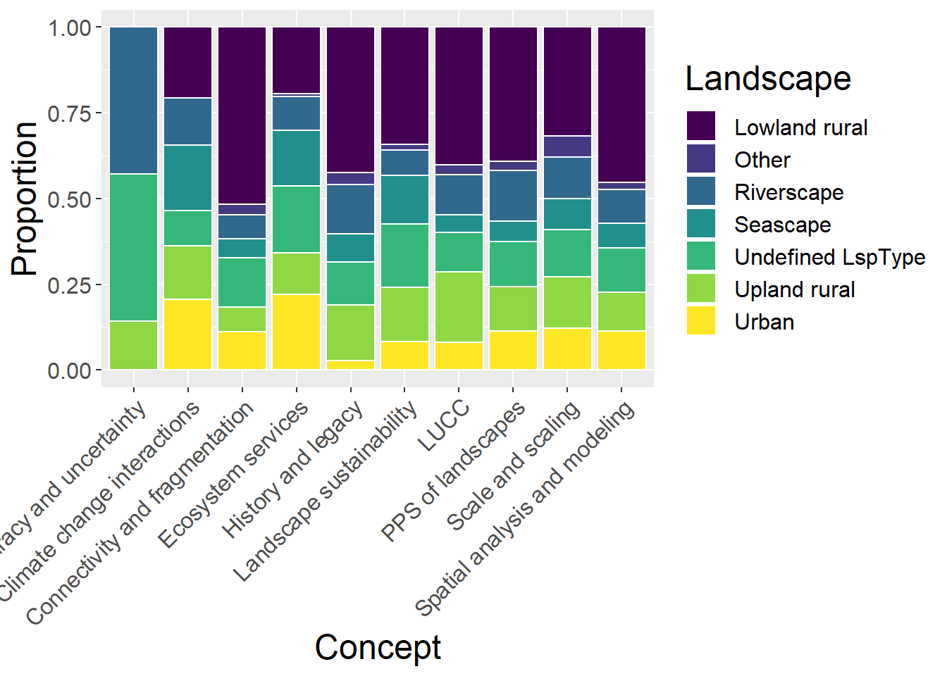

9.3.2 Without ‘Undefined LspType’ and ‘Other’ landscape types

General observations:

Patterns seen above more obvious

lspCounts <- conceptdata %>%
  select(Concept,`Upland rural`, `Lowland rural`, Urban,    Riverscape, Seascape) %>%
  mutate(sum = rowSums(.[2:6])) %>%   #calculate total for subsquent calcultation of proportion
  gather(key = Type, value = count, -Concept, -sum) %>%
  mutate(prop = count / sum)  #calculate proportion

conceptdata %>%
  select(Concept,`Upland rural`, `Lowland rural`, Urban,    Riverscape, Seascape) %>%
  mutate(Total = rowSums(.[2:6])) %>%   #calculate total
  mutate_if(is.numeric, funs(prop = ./ Total)) %>%
  mutate_at(vars(ends_with("prop")), round, 3) %>% 
  select(-Total_prop) %>%
  kable() %>%
  kable_styling() %>%
  scroll_box(width = "100%")

Concept	Upland rural	Lowland rural	Urban	Riverscape	Seascape	Total	Upland rural_prop	Lowland rural_prop	Urban_prop	Riverscape_prop	Seascape_prop
Accuracy and uncertainty	1	0	0	3	0	4	0.250	0.000	0.000	0.750	0.000
Climate change interactions	9	12	12	8	11	52	0.173	0.231	0.231	0.154	0.212
Connectivity and fragmentation	16	112	24	15	12	179	0.089	0.626	0.134	0.084	0.067
Ecosystem services	15	24	27	12	20	98	0.153	0.245	0.276	0.122	0.204
History and legacy	18	47	3	16	9	93	0.194	0.505	0.032	0.172	0.097
Landscape sustainability	19	41	10	9	17	96	0.198	0.427	0.104	0.094	0.177
LUCC	56	109	22	32	14	233	0.240	0.468	0.094	0.137	0.060
PPS of landscapes	15	45	13	17	7	97	0.155	0.464	0.134	0.175	0.072
Scale and scaling	10	21	8	8	6	53	0.189	0.396	0.151	0.151	0.113
Spatial analysis and modeling	22	88	22	19	14	165	0.133	0.533	0.133	0.115	0.085

ggplot(lspCounts, aes(x=Concept, y=count, fill=Type)) + 
  geom_bar(stat="identity", colour="white") + 
  theme(axis.text.x = element_text(angle = 45, hjust = 1)) +
  scale_fill_viridis(discrete = TRUE) +
  labs(fill="Landscape", y = "Abstract Count", x="Concept")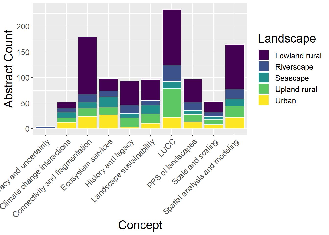

ggplot(lspCounts, aes(x=Concept, y=prop, fill=Type)) + 
  geom_bar(stat="identity", colour="white") + 
  theme(axis.text.x = element_text(angle = 45, hjust = 1)) +
  scale_fill_viridis(discrete = TRUE) +
  labs(fill="Landscape", y = "Proportion", x="Concept")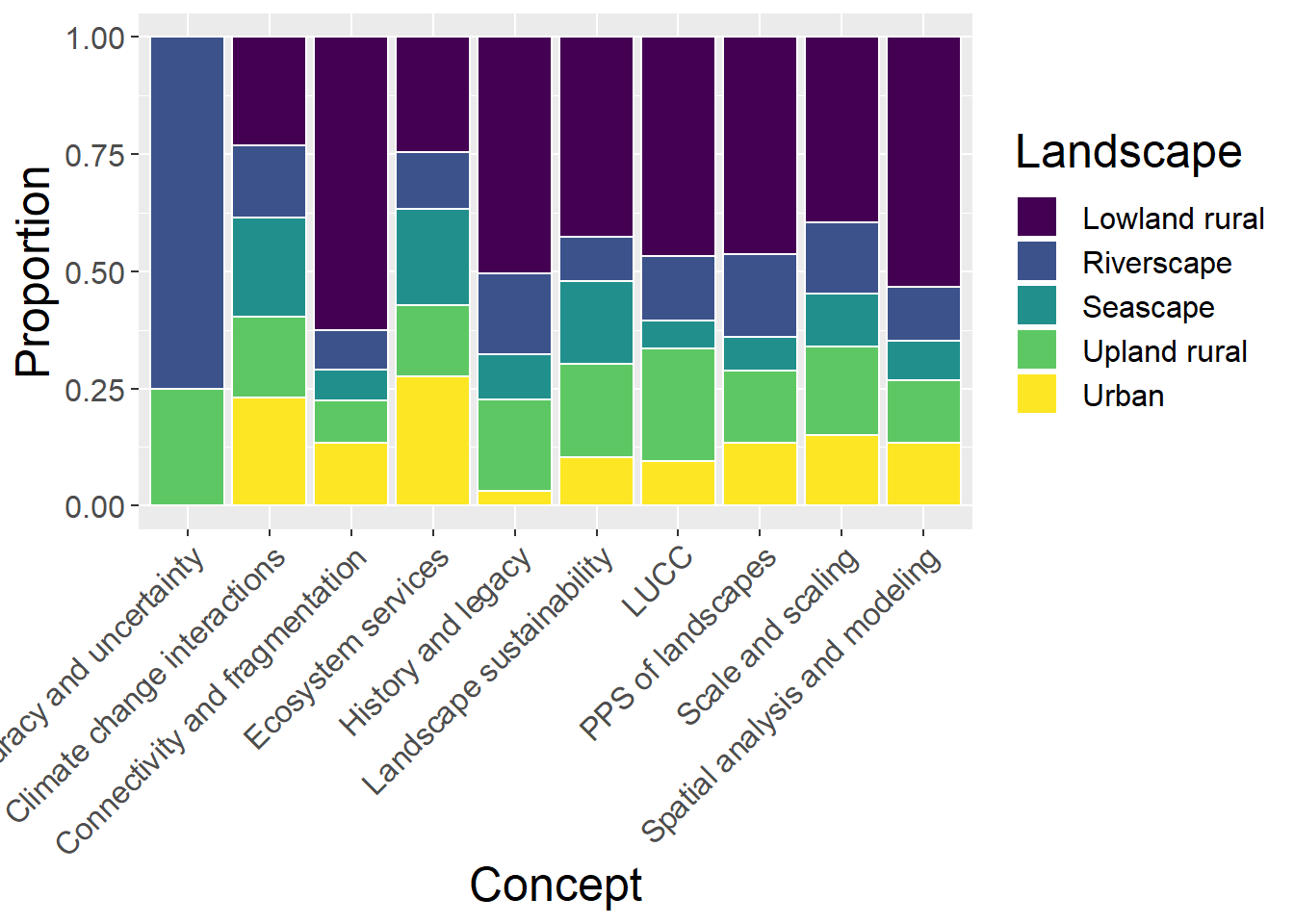

9.4 Organism

General observations

Ecosystem services have greatest proportion of humans (31%)

speciesCounts <- conceptdata %>%
  select(Concept, Mammals, Humans, Birds, Reptiles, Inverts, Plants, Amphibians, Fish, `Generic Habitat`,`Woodland Forests`) %>%
  mutate(sum = rowSums(.[2:11])) %>%   #calculate total for subsquent calcultation of proportion
  gather(key = Type, value = count, -Concept, -sum) %>%
  mutate(prop = count / sum)  #calculate proportion

conceptdata %>%
  select(Concept, Mammals, Humans, Birds, Reptiles, Inverts, Plants, Amphibians, Fish, `Generic Habitat`,`Woodland Forests`) %>%
  mutate(Total = rowSums(.[2:11])) %>%   #calculate total for subsquent calcultation of proportion
  mutate_if(is.numeric, funs(prop = ./ Total)) %>%
  mutate_at(vars(ends_with("prop")), round, 3) %>% 
  select(-Total_prop) %>%
  kable() %>%
  kable_styling() %>%
  scroll_box(width = "100%")

Concept	Mammals	Humans	Birds	Reptiles	Inverts	Plants	Amphibians	Fish	Generic Habitat	Woodland Forests	Total	Mammals_prop	Humans_prop	Birds_prop	Reptiles_prop	Inverts_prop	Plants_prop	Amphibians_prop	Fish_prop	Generic Habitat_prop	Woodland Forests_prop
Accuracy and uncertainty	0	0	0	0	0	2	0	0	3	1	6	0.000	0.000	0.000	0.000	0.000	0.333	0.000	0.000	0.500	0.167
Climate change interactions	2	12	2	1	2	7	0	1	13	10	50	0.040	0.240	0.040	0.020	0.040	0.140	0.000	0.020	0.260	0.200
Connectivity and fragmentation	19	4	40	1	37	25	4	3	53	57	243	0.078	0.016	0.165	0.004	0.152	0.103	0.016	0.012	0.218	0.235
Ecosystem services	1	29	5	1	6	6	0	2	28	15	93	0.011	0.312	0.054	0.011	0.065	0.065	0.000	0.022	0.301	0.161
History and legacy	4	19	9	1	7	15	1	1	42	25	124	0.032	0.153	0.073	0.008	0.056	0.121	0.008	0.008	0.339	0.202
Landscape sustainability	2	26	10	1	3	7	0	1	20	20	90	0.022	0.289	0.111	0.011	0.033	0.078	0.000	0.011	0.222	0.222
LUCC	6	29	27	3	15	35	4	2	92	52	265	0.023	0.109	0.102	0.011	0.057	0.132	0.015	0.008	0.347	0.196
PPS of landscapes	7	4	24	1	31	21	1	5	34	16	144	0.049	0.028	0.167	0.007	0.215	0.146	0.007	0.035	0.236	0.111
Scale and scaling	6	5	16	0	12	5	0	1	17	9	71	0.085	0.070	0.225	0.000	0.169	0.070	0.000	0.014	0.239	0.127
Spatial analysis and modeling	10	11	39	0	27	21	1	0	56	40	205	0.049	0.054	0.190	0.000	0.132	0.102	0.005	0.000	0.273	0.195

ggplot(speciesCounts, aes(x=Concept, y=count, fill=Type)) + 
  geom_bar(stat="identity", colour="white") + 
  theme(axis.text.x = element_text(angle = 45, hjust = 1)) +
  scale_fill_viridis(discrete = TRUE) +
  labs(fill="Organism", y = "Abstract Count", x="Concept")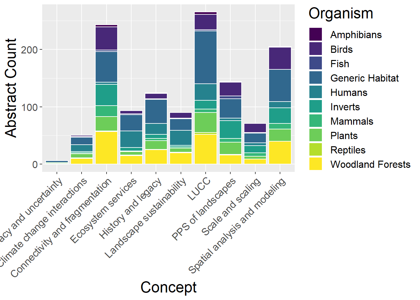

ggplot(speciesCounts, aes(x=Concept, y=prop, fill=Type)) + 
  geom_bar(stat="identity", colour="white") + 
  theme(axis.text.x = element_text(angle = 45, hjust = 1)) +
  scale_fill_viridis(discrete = TRUE) +
  labs(fill="Organism", y = "Proportion", x="Concept")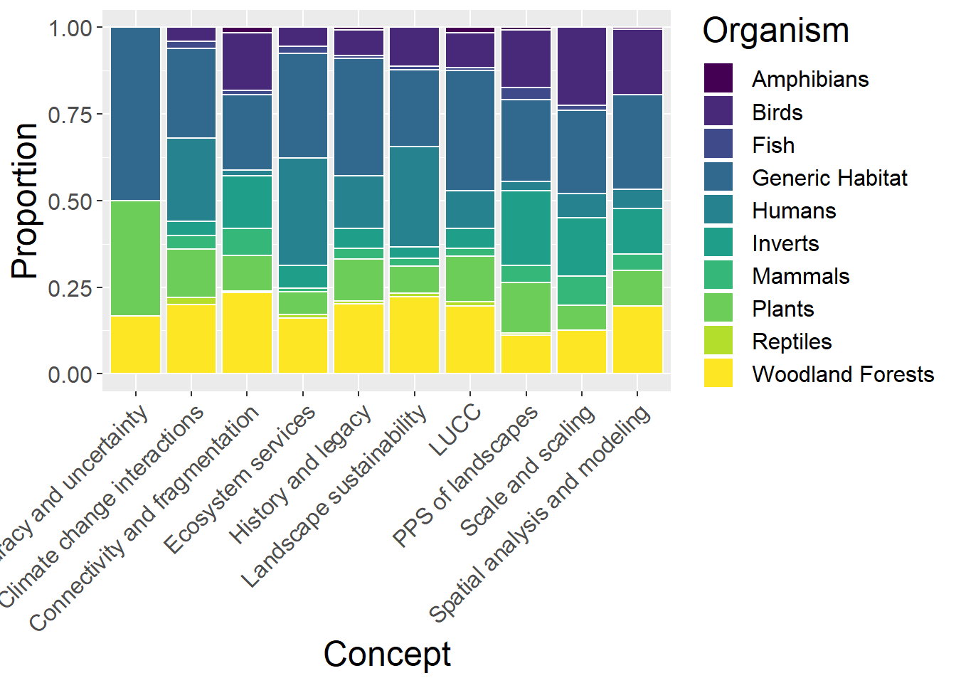

9.5 Methods

General observations:

Ecosystem services has smallest proportion of Empirical studies

methodsCounts <- conceptdata %>%
  select(Concept, Empirical, Theoretical, Qualitative, Quantitative, GIS, `Remote sensing`) %>%
  mutate(sum = rowSums(.[2:7])) %>%
  gather(key = Type, value = count, -Concept, -sum) %>%
  mutate(prop = count / sum) 

conceptdata %>%
  select(Concept, Empirical, Theoretical, Qualitative, Quantitative, GIS, `Remote sensing`) %>%
  mutate(Total = rowSums(.[2:7])) %>%
  mutate_if(is.numeric, funs(prop = ./ Total)) %>%
  mutate_at(vars(ends_with("prop")), round, 3) %>% 
  select(-Total_prop) %>%
  kable() %>%
  kable_styling() %>%
  scroll_box(width = "100%")

Concept	Empirical	Theoretical	Qualitative	Quantitative	GIS	Remote sensing	Total	Empirical_prop	Theoretical_prop	Qualitative_prop	Quantitative_prop	GIS_prop	Remote sensing_prop
Accuracy and uncertainty	2	2	0	5	0	0	9	0.222	0.222	0.000	0.556	0.000	0.000
Climate change interactions	10	16	13	21	14	2	76	0.132	0.211	0.171	0.276	0.184	0.026
Connectivity and fragmentation	113	43	18	92	55	10	331	0.341	0.130	0.054	0.278	0.166	0.030
Ecosystem services	14	38	36	43	30	4	165	0.085	0.230	0.218	0.261	0.182	0.024
History and legacy	41	21	30	38	18	6	154	0.266	0.136	0.195	0.247	0.117	0.039
Landscape sustainability	30	31	40	33	15	0	149	0.201	0.208	0.268	0.221	0.101	0.000
LUCC	98	47	53	107	66	18	389	0.252	0.121	0.136	0.275	0.170	0.046
PPS of landscapes	69	16	8	58	23	12	186	0.371	0.086	0.043	0.312	0.124	0.065
Scale and scaling	34	11	6	35	12	9	107	0.318	0.103	0.056	0.327	0.112	0.084
Spatial analysis and modeling	78	35	21	117	96	16	363	0.215	0.096	0.058	0.322	0.264	0.044

ggplot(methodsCounts, aes(x=Concept, y=count, fill=Type)) + 
  geom_bar(stat="identity", colour="white") + 
  theme(axis.text.x = element_text(angle = 45, hjust = 1))  +
  scale_fill_viridis(discrete = TRUE) +
  labs(fill="Method", y = "Abstract Count", x="Concept")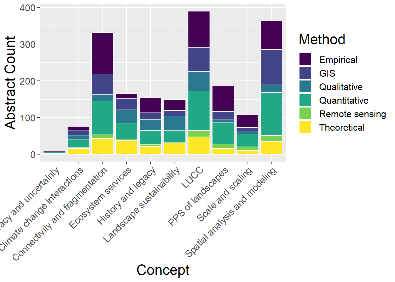

ggplot(methodsCounts, aes(x=Concept, y=prop, fill=Type)) + 
  geom_bar(stat="identity", colour="white") + 
  theme(axis.text.x = element_text(angle = 45, hjust = 1)) +
  scale_fill_viridis(discrete = TRUE) +
  labs(fill="Method", y = "Proportion", x="Concept")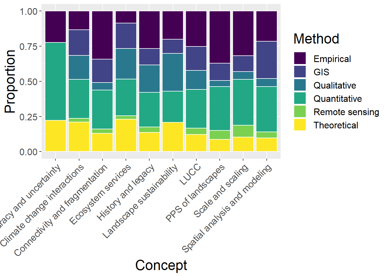

9.6 Spatial Extent

General observations:

Ecosystem services has the largest proportion of global studies and fewest mini and micro studies
Connectivity & Fragmentation has largest proportion of local studies

spatialCounts <- conceptdata %>%
  select(Concept, Micro, Mini, Local, Regional, National, Continental, Global,`Undefined Extent`) %>%
  mutate(sum = rowSums(.[2:9])) %>%
  gather(key = Type, value = count, -Concept, -sum) %>%
  mutate(prop = count / sum) 

conceptdata %>%
  select(Concept, Micro, Mini, Local, Regional, National, Continental, Global,`Undefined Extent`) %>%
  mutate(Total = rowSums(.[2:9])) %>%
  mutate_if(is.numeric, funs(prop = ./ Total)) %>%
  mutate_at(vars(ends_with("prop")), round, 3) %>% 
  select(-Total_prop) %>%
  kable() %>%
  kable_styling() %>%
  scroll_box(width = "100%")

Concept	Micro	Mini	Local	Regional	National	Continental	Global	Undefined Extent	Total	Micro_prop	Mini_prop	Local_prop	Regional_prop	National_prop	Continental_prop	Global_prop	Undefined Extent_prop
Accuracy and uncertainty	0	1	2	1	2	0	0	1	7	0.000	0.143	0.286	0.143	0.286	0.000	0.000	0.143
Climate change interactions	0	4	15	15	8	1	2	5	50	0.000	0.080	0.300	0.300	0.160	0.020	0.040	0.100
Connectivity and fragmentation	7	25	71	48	25	4	2	30	212	0.033	0.118	0.335	0.226	0.118	0.019	0.009	0.142
Ecosystem services	1	6	33	22	25	5	6	22	120	0.008	0.050	0.275	0.183	0.208	0.042	0.050	0.183
History and legacy	0	8	25	30	22	5	2	5	97	0.000	0.082	0.258	0.309	0.227	0.052	0.021	0.052
Landscape sustainability	0	7	27	27	21	6	2	13	103	0.000	0.068	0.262	0.262	0.204	0.058	0.019	0.126
LUCC	7	20	73	62	59	13	3	15	252	0.028	0.079	0.290	0.246	0.234	0.052	0.012	0.060
PPS of landscapes	11	20	33	19	12	1	2	16	114	0.096	0.175	0.289	0.167	0.105	0.009	0.018	0.140
Scale and scaling	6	12	18	10	8	2	1	9	66	0.091	0.182	0.273	0.152	0.121	0.030	0.015	0.136
Spatial analysis and modeling	7	16	67	58	31	7	1	21	208	0.034	0.077	0.322	0.279	0.149	0.034	0.005	0.101

factor_order <- c('Micro', 'Mini', 'Local', 'Regional', 'National', 'Continental', 'Global','Undefined Extent')
factor_labels <- c('Micro', 'Mini', 'Local', 'Regional', 'National', 'Continental', 'Global','Undefined')

ggplot(spatialCounts, aes(x=Concept, y=count, fill=factor(Type, level=factor_order))) + 
  geom_bar(stat="identity", colour="white") + 
  theme(axis.text.x = element_text(angle = 45, hjust = 1))  +
  scale_fill_viridis(discrete = TRUE) +
  labs(fill="Spatial", y = "Abstract Count", x="Concept")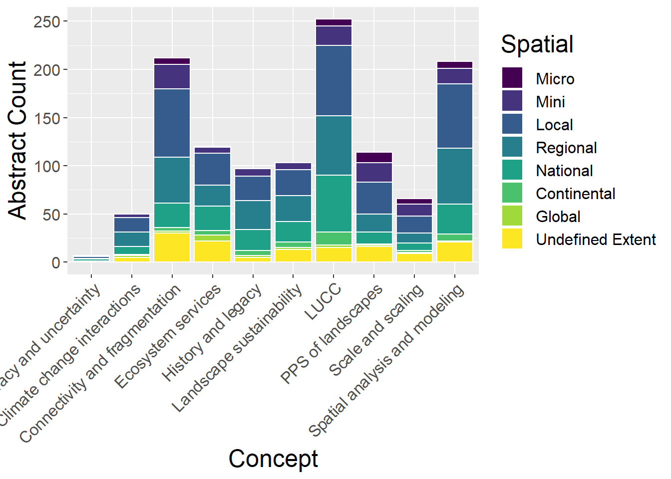

ggplot(spatialCounts, aes(x=Concept, y=prop, fill=factor(Type, level=factor_order))) + 
  geom_bar(stat="identity", colour="white") + 
  theme(axis.text.x = element_text(angle = 45, hjust = 1)) +
  scale_fill_viridis(discrete = TRUE) +
  labs(fill="Spatial", y = "Proportion", x="Concept")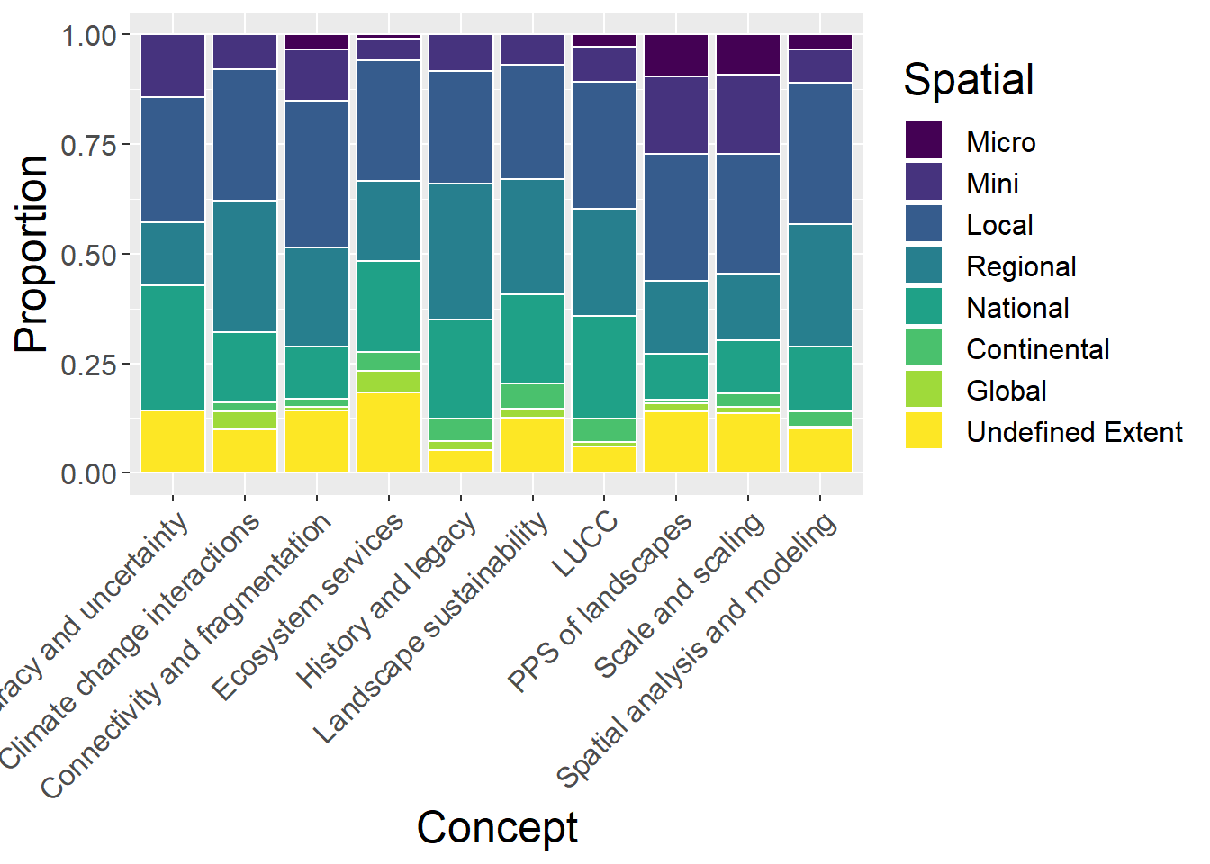

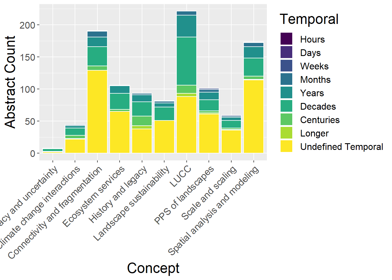
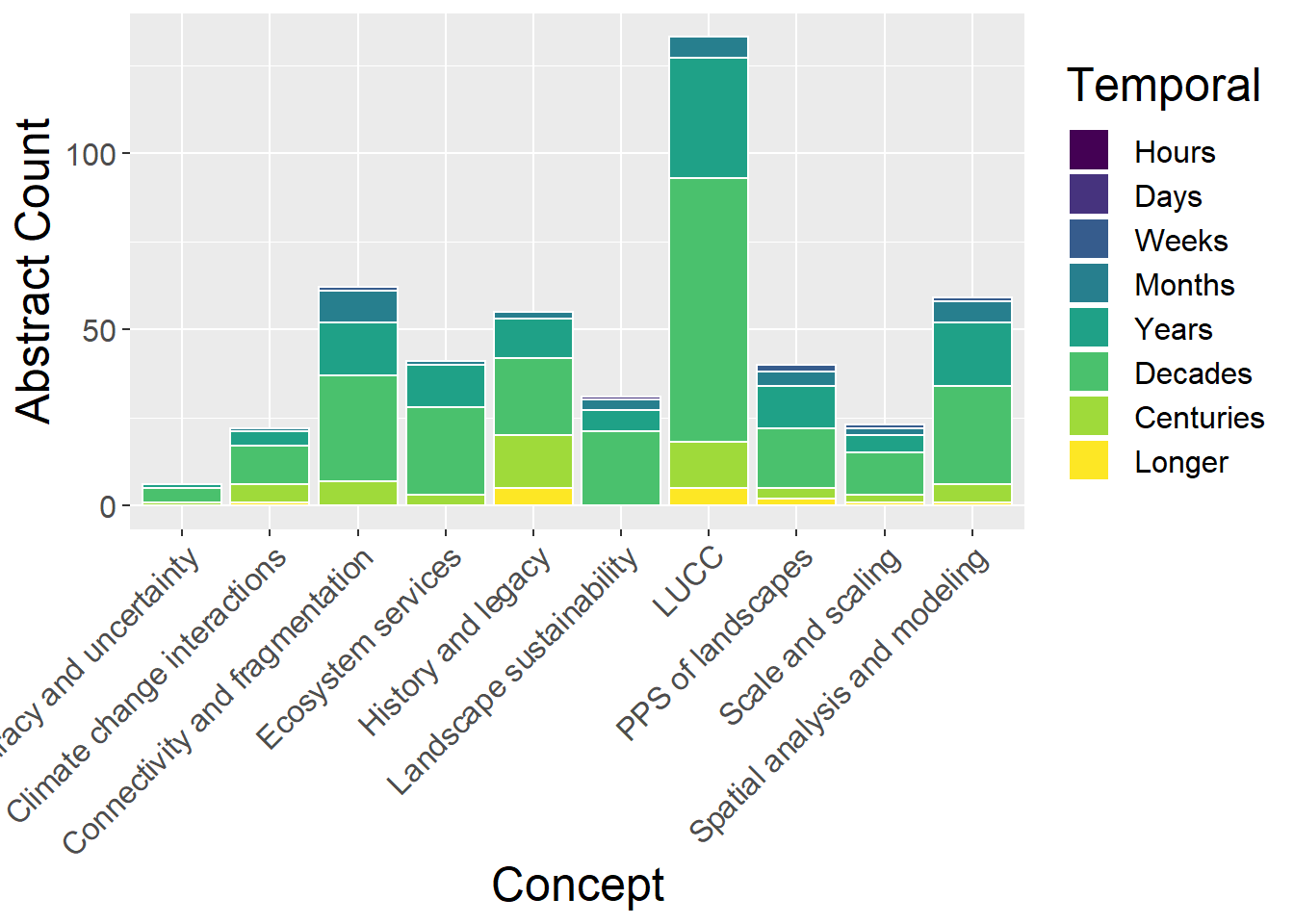
9.7 Temporal Extent

9.7.1 With undefined

General observations:

Concept	Days	Weeks	Months	Years	Decades	Centuries	Longer	Undefined Temporal	Total	Days_prop	Weeks_prop	Months_prop	Years_prop	Decades_prop	Centuries_prop	Longer_prop	Undefined Temporal_prop
Accuracy and uncertainty	0	0	0	1	4	1	0	2	8	0.000	0.000	0.000	0.125	0.500	0.125	0.000	0.250
Climate change interactions	0	0	1	4	11	5	1	22	44	0.000	0.000	0.023	0.091	0.250	0.114	0.023	0.500
Connectivity and fragmentation	0	1	9	15	30	7	0	129	191	0.000	0.005	0.047	0.079	0.157	0.037	0.000	0.675
Ecosystem services	0	0	1	12	25	3	0	65	106	0.000	0.000	0.009	0.113	0.236	0.028	0.000	0.613
History and legacy	0	0	2	11	22	15	5	38	93	0.000	0.000	0.022	0.118	0.237	0.161	0.054	0.409
Landscape sustainability	1	0	3	6	21	0	0	51	82	0.012	0.000	0.037	0.073	0.256	0.000	0.000	0.622
LUCC	0	0	6	34	75	13	5	88	221	0.000	0.000	0.027	0.154	0.339	0.059	0.023	0.398
PPS of landscapes	0	2	4	12	17	3	2	61	101	0.000	0.020	0.040	0.119	0.168	0.030	0.020	0.604
Scale and scaling	0	1	2	5	12	2	1	36	59	0.000	0.017	0.034	0.085	0.203	0.034	0.017	0.610
Spatial analysis and modeling	0	1	6	18	28	5	1	114	173	0.000	0.006	0.035	0.104	0.162	0.029	0.006	0.659

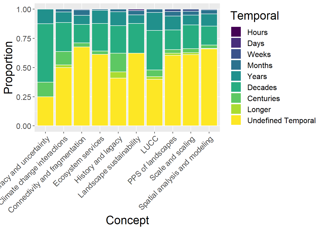
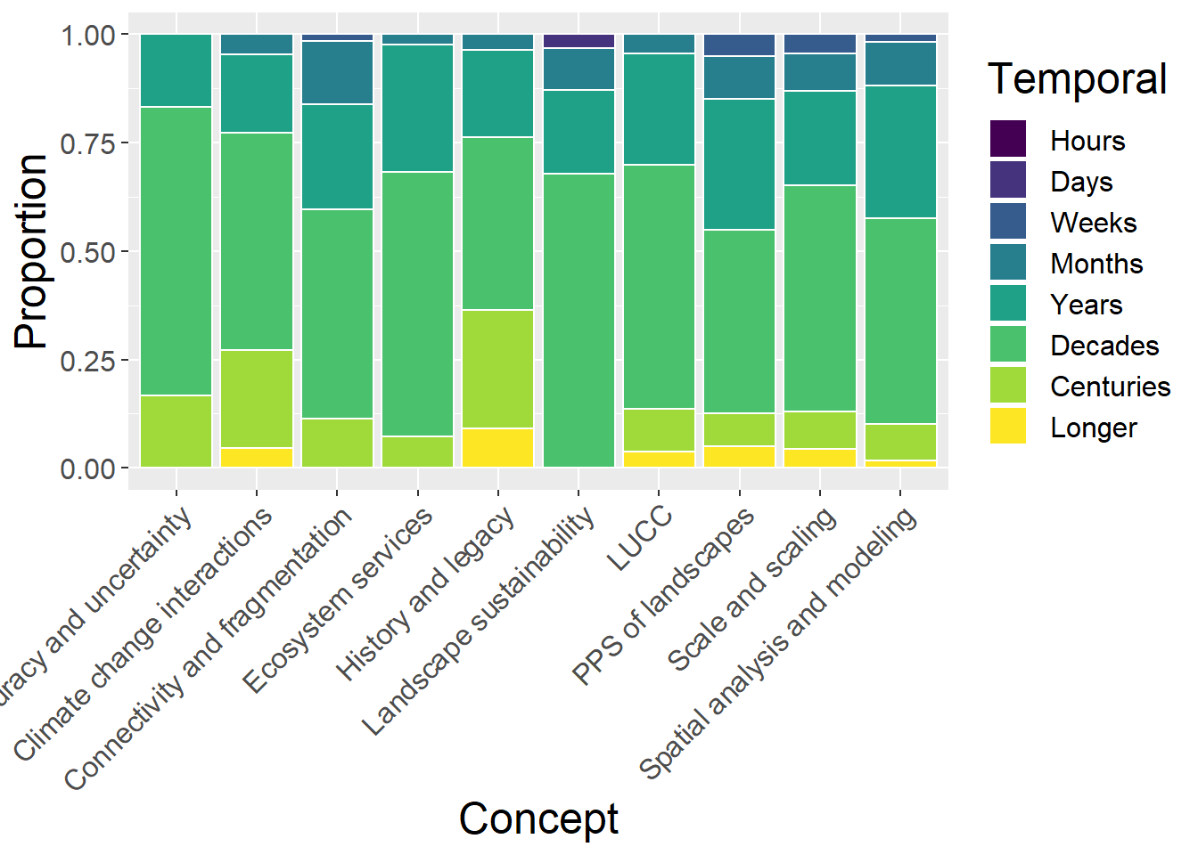
9.7.2 Without Undefined

History and Legacy studies have greatest proportion of Centries and Longer studies

Concept	Days	Weeks	Months	Years	Decades	Centuries	Longer	Total	Days_prop	Weeks_prop	Months_prop	Years_prop	Decades_prop	Centuries_prop	Longer_prop
Accuracy and uncertainty	0	0	0	1	4	1	0	6	0.000	0.000	0.000	0.167	0.667	0.167	0.000
Climate change interactions	0	0	1	4	11	5	1	22	0.000	0.000	0.045	0.182	0.500	0.227	0.045
Connectivity and fragmentation	0	1	9	15	30	7	0	62	0.000	0.016	0.145	0.242	0.484	0.113	0.000
Ecosystem services	0	0	1	12	25	3	0	41	0.000	0.000	0.024	0.293	0.610	0.073	0.000
History and legacy	0	0	2	11	22	15	5	55	0.000	0.000	0.036	0.200	0.400	0.273	0.091
Landscape sustainability	1	0	3	6	21	0	0	31	0.032	0.000	0.097	0.194	0.677	0.000	0.000
LUCC	0	0	6	34	75	13	5	133	0.000	0.000	0.045	0.256	0.564	0.098	0.038
PPS of landscapes	0	2	4	12	17	3	2	40	0.000	0.050	0.100	0.300	0.425	0.075	0.050
Scale and scaling	0	1	2	5	12	2	1	23	0.000	0.043	0.087	0.217	0.522	0.087	0.043
Spatial analysis and modeling	0	1	6	18	28	5	1	59	0.000	0.017	0.102	0.305	0.475	0.085	0.017

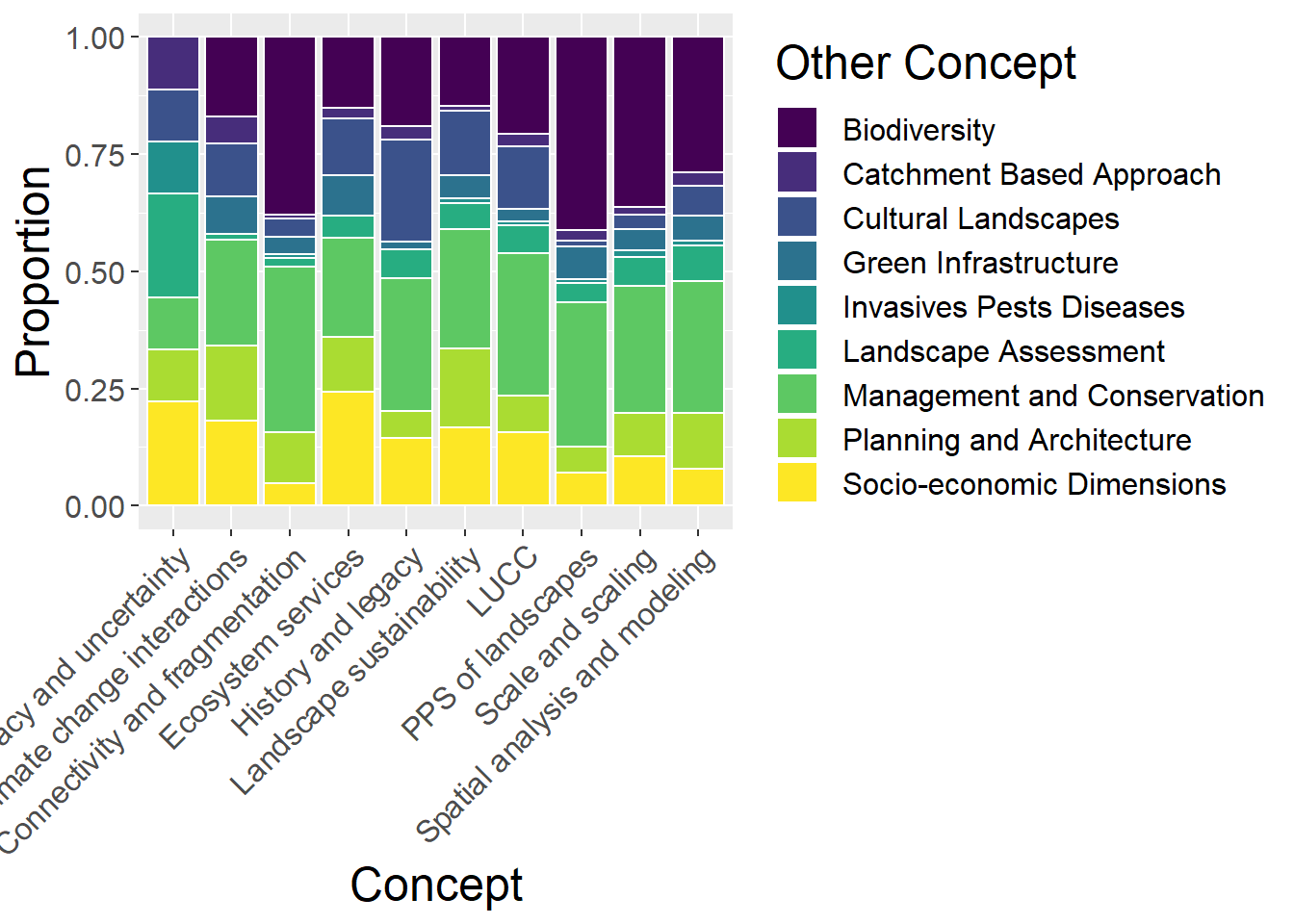
9.8 Other Concepts

General observations:

Connectivity & Fragmentation and pattern-process-scale have greatest proportion of biodiversity studies
History and Legacy have greatest proportion of cultural studies

otherCounts <- conceptdata %>%
  select(Concept, `Green Infrastructure`,`Planning and Architecture`,`Management and Conservation`,`Cultural Landscapes`,`Socio-economic Dimensions`,Biodiversity,`Landscape Assessment`,`Catchment Based Approach`,`Invasives Pests Diseases`
) %>%
  mutate(sum = rowSums(.[2:10])) %>%
  gather(key = Type, value = count, -Concept, -sum) %>%
  mutate(prop = count / sum) 

conceptdata %>%
  select(Concept, `Green Infrastructure`,`Planning and Architecture`,`Management and Conservation`,`Cultural Landscapes`,`Socio-economic Dimensions`,Biodiversity,`Landscape Assessment`,`Catchment Based Approach`,`Invasives Pests Diseases`
) %>%
  mutate(Total = rowSums(.[2:10])) %>%
  mutate_if(is.numeric, funs(prop = ./ Total)) %>%
  mutate_at(vars(ends_with("prop")), round, 3) %>% 
  select(-Total_prop) %>%
  kable() %>%
  kable_styling() %>%
  scroll_box(width = "100%")

Concept	Green Infrastructure	Planning and Architecture	Management and Conservation	Cultural Landscapes	Socio-economic Dimensions	Biodiversity	Landscape Assessment	Catchment Based Approach	Invasives Pests Diseases	Total	Green Infrastructure_prop	Planning and Architecture_prop	Management and Conservation_prop	Cultural Landscapes_prop	Socio-economic Dimensions_prop	Biodiversity_prop	Landscape Assessment_prop	Catchment Based Approach_prop	Invasives Pests Diseases_prop
Accuracy and uncertainty	0	1	1	1	2	0	2	1	1	9	0.000	0.111	0.111	0.111	0.222	0.000	0.222	0.111	0.111
Climate change interactions	7	14	20	10	16	15	1	5	0	88	0.080	0.159	0.227	0.114	0.182	0.170	0.011	0.057	0.000
Connectivity and fragmentation	10	30	97	11	13	104	5	2	2	274	0.036	0.109	0.354	0.040	0.047	0.380	0.018	0.007	0.007
Ecosystem services	20	27	49	28	56	35	11	5	0	231	0.087	0.117	0.212	0.121	0.242	0.152	0.048	0.022	0.000
History and legacy	3	10	51	39	26	34	11	5	0	179	0.017	0.056	0.285	0.218	0.145	0.190	0.061	0.028	0.000
Landscape sustainability	10	34	52	28	34	30	11	2	2	203	0.049	0.167	0.256	0.138	0.167	0.148	0.054	0.010	0.010
LUCC	9	27	104	46	54	71	21	9	3	344	0.026	0.078	0.302	0.134	0.157	0.206	0.061	0.026	0.009
PPS of landscapes	10	8	44	2	10	59	6	3	1	143	0.070	0.056	0.308	0.014	0.070	0.413	0.042	0.021	0.007
Scale and scaling	3	6	18	2	7	24	4	1	1	66	0.045	0.091	0.273	0.030	0.106	0.364	0.061	0.015	0.015
Spatial analysis and modeling	14	32	75	17	21	77	20	8	3	267	0.052	0.120	0.281	0.064	0.079	0.288	0.075	0.030	0.011

ggplot(otherCounts, aes(x=Concept, y=count, fill=Type)) + 
  geom_bar(stat="identity", colour="white") + 
  theme(axis.text.x = element_text(angle = 45, hjust = 1))  +
  scale_fill_viridis(discrete = TRUE) +
  labs(fill="Other Concept", y = "Abstract Count", x="Concept")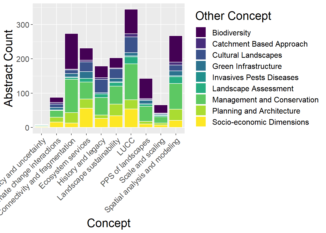

ggplot(otherCounts, aes(x=Concept, y=prop, fill=Type)) + 
  geom_bar(stat="identity", colour="white") + 
  theme(axis.text.x = element_text(angle = 45, hjust = 1)) +
  scale_fill_viridis(discrete = TRUE) +
  labs(fill="Other Concept", y = "Proportion", x="Concept")