Chapter 6 Analysis by Methods

Bar charts and tables to examine how contributions to conferences vary by methods

#spec(cpdata)

metdata <- cpdata %>%
  select_if(is.numeric) %>%
  gather(key = Method, value = count, Empirical:`Remote sensing`) %>%
  filter(count > 0) %>%
  group_by(`Method`) %>%
  summarise_all(sum, na.rm=T) 

6.1 Total Conference Contributions

General observations:

• Empirical and Quantitative studies dominate
• little remote sensing

metdata %>%
  select(Method, count) %>%
  mutate(prop = count/sum(count)) %>%
  mutate(prop = round(prop,3)) %>% 
  kable() %>%
  kable_styling() %>%
  scroll_box(width = "100%")

Method	count	prop
Empirical	375	0.292
GIS	185	0.144
Qualitative	154	0.120
Quantitative	351	0.273
Remote sensing	41	0.032
Theoretical	178	0.139

ggplot(metdata, aes(x=Method, y=count)) + 
  geom_bar(stat="identity") + 
  geom_text(aes(x=Method, y=max(count), label = paste0(round(100*count / sum(count),1), "%"), vjust=-0.25)) + theme(axis.text.x = element_text(angle = 30, hjust = 1)) +
  labs(y = "Abstract Count")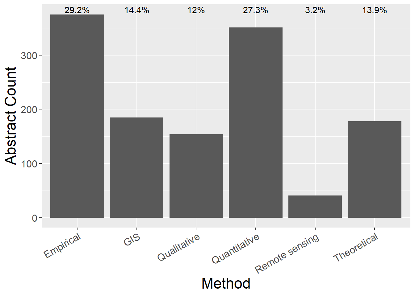

6.2 Author Affiliation

General observations:

• Pretty consistent distribution of methods across affiliations

authorCounts <- metdata %>%
  select(Method,Academic, Government,NGO,Business,Private) %>%
  mutate(sum = rowSums(.[2:6])) %>%   #calculate total for subsquent calcultation of proportion
  gather(key = Type, value = count, -Method, -sum) %>%
  mutate(prop = count / sum)  #calculate proportion


ggplot(authorCounts, aes(x=Method, y=count, fill=Type)) + geom_bar(stat="identity", colour="white")  +
  scale_fill_viridis(discrete = TRUE) +
  theme(axis.text.x = element_text(angle = 30, hjust = 1)) +
  labs(fill="Affiliation", y = "Abstract Count", x="Method")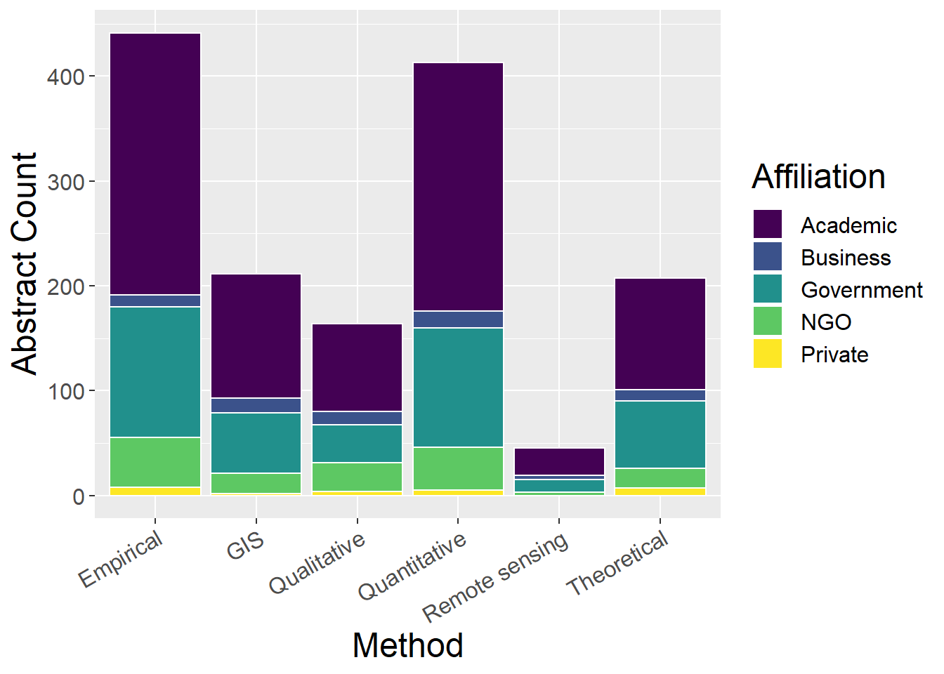

ggplot(authorCounts, aes(x=Method, y=prop, fill=Type)) + geom_bar(stat="identity", colour="white")  +
  scale_fill_viridis(discrete = TRUE) +
  theme(axis.text.x = element_text(angle = 30, hjust = 1)) +
  labs(fill="Affiliation", y = "Proportion", x="Method")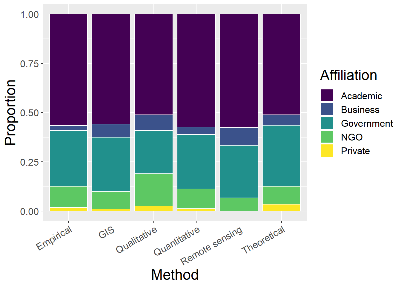

6.3 Landscape Type

6.3.1 Using all landscape types

General observations:

• Qualitative studies are most evenly distributed across landscape types
• Theoretical studies most commonly do not define a landscape type

lspCounts <- metdata %>%
  select(Method,`Upland rural`, `Lowland rural`, Urban, Riverscape, Seascape, `Undefined LspType`,Other) %>%
  mutate(sum = rowSums(.[2:8])) %>%   #calculate total for subsquent calcultation of proportion
  gather(key = Type, value = count, -Method, -sum) %>%
  mutate(prop = count / sum)  #calculate proportion

ggplot(lspCounts, aes(x=Method, y=count, fill=Type)) + geom_bar(stat="identity", colour="white")  +
  scale_fill_viridis(discrete = TRUE) +
  theme(axis.text.x = element_text(angle = 30, hjust = 1)) +
  labs(fill="Landscape Type", y = "Abstract Count", x="Method")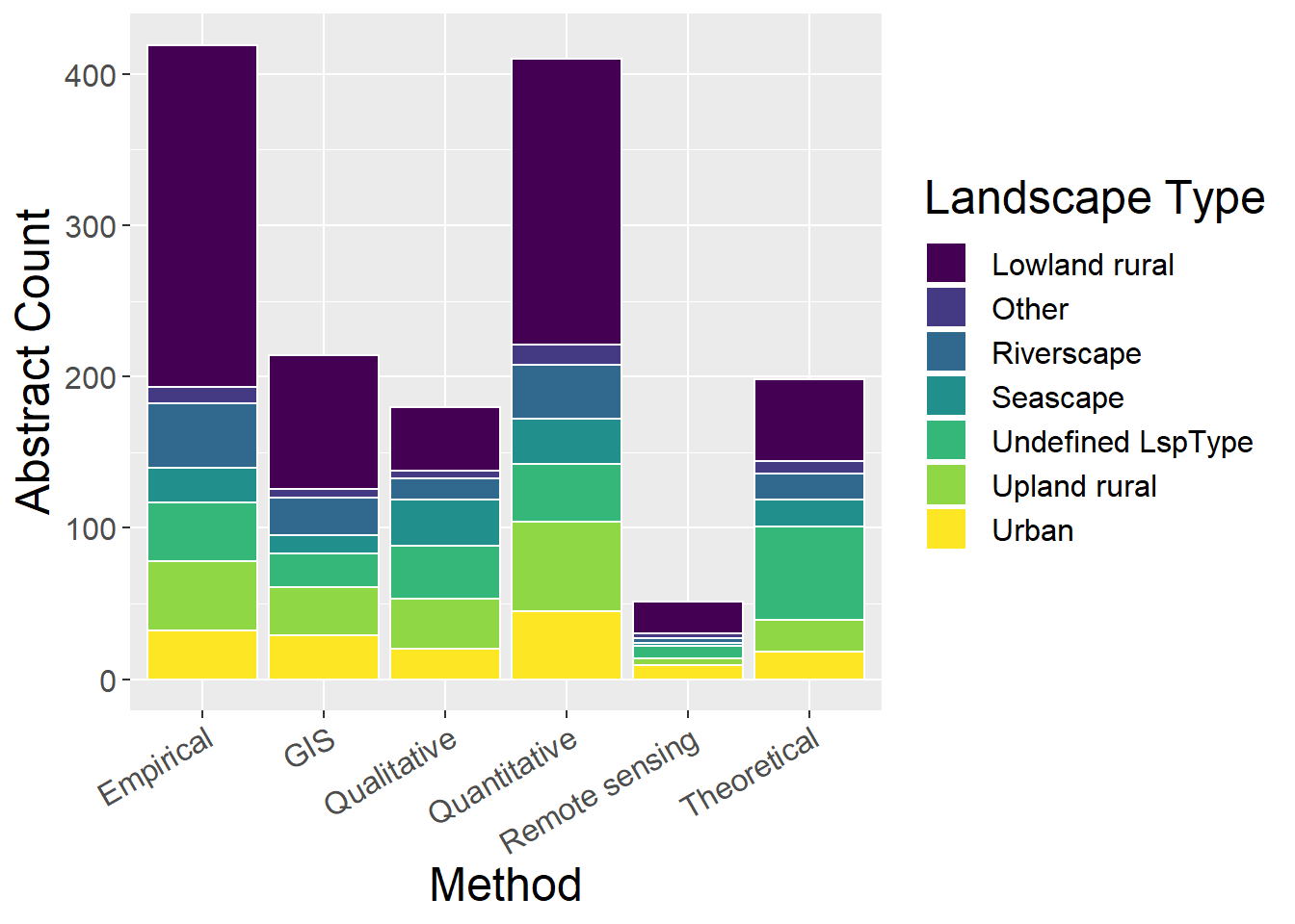

ggplot(lspCounts, aes(x=Method, y=prop, fill=Type)) + geom_bar(stat="identity", colour="white")  +
  scale_fill_viridis(discrete = TRUE) +
  theme(axis.text.x = element_text(angle = 30, hjust = 1)) +
  labs(fill="Landscape Type", y = "Proportion", x="Method")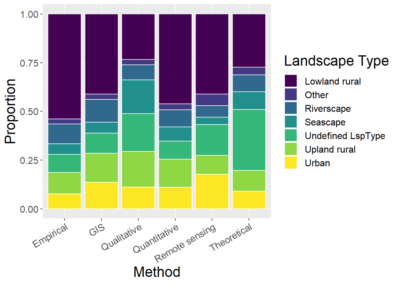

6.3.2 Without ‘Undefined LspType’ and ‘Other’ landscape types

General observations:

• This is generally less informative than with ‘un-defined’ (in contrast to other classifications)
• Does highlight that qualitative studies are most prevalent in seascape studies

lspCounts <- metdata %>%
  select(Method,`Upland rural`, `Lowland rural`, Urban, Riverscape, Seascape) %>%
  mutate(sum = rowSums(.[2:6])) %>%   #calculate total for subsquent calcultation of proportion
  gather(key = Type, value = count, -Method, -sum) %>%
  mutate(prop = count / sum)  #calculate proportion

ggplot(lspCounts, aes(x=Method, y=count, fill=Type)) + geom_bar(stat="identity", colour="white")  +
  scale_fill_viridis(discrete = TRUE) +
  theme(axis.text.x = element_text(angle = 30, hjust = 1)) +
  labs(fill="Landscape", y = "Abstract Count", x="Method")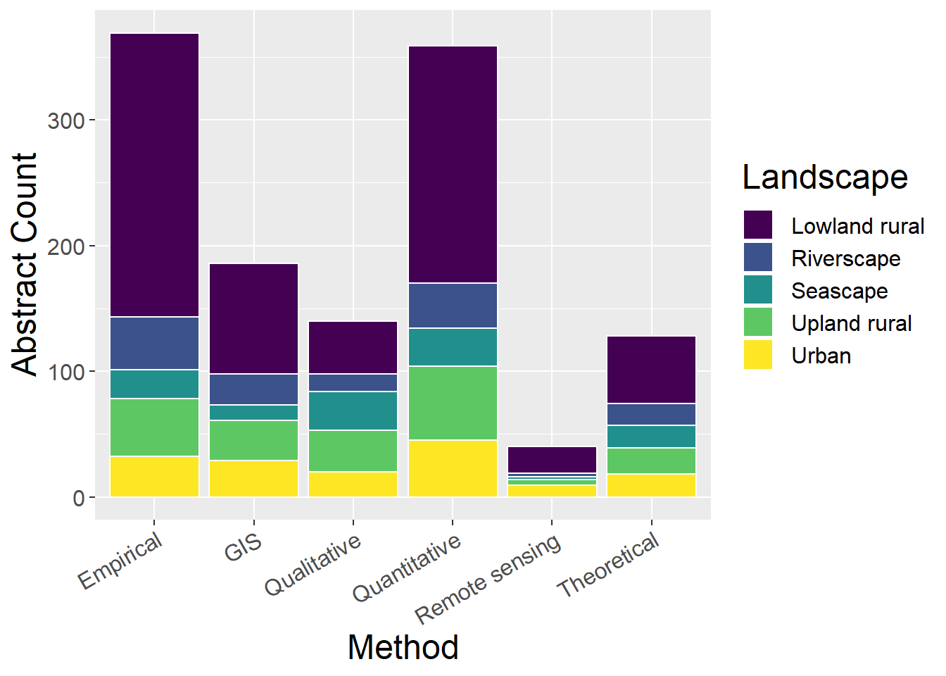

ggplot(lspCounts, aes(x=Method, y=prop, fill=Type)) + geom_bar(stat="identity", colour="white")  +
  scale_fill_viridis(discrete = TRUE) +
  theme(axis.text.x = element_text(angle = 30, hjust = 1)) +
  labs(fill="Landscape", y = "Proportion", x="Method")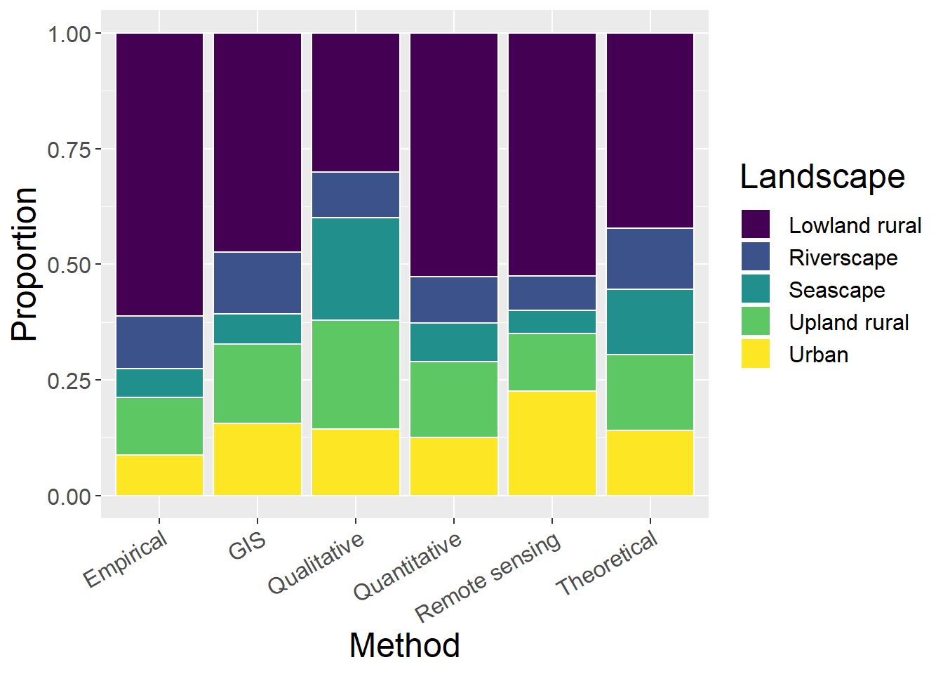

6.4 Organism

General observations

• Qualitative studies most commonly study humans

sppCounts <- metdata %>%
  select(Method,Mammals, Humans, Birds, Reptiles, Inverts, Plants, Amphibians, Fish, `Generic Habitat`,`Woodland Forests`) %>%
  mutate(sum = rowSums(.[2:11])) %>%   #calculate total for subsquent calcultation of proportion
  gather(key = Type, value = count, -Method, -sum) %>%
  mutate(prop = count / sum)  #calculate proportion

ggplot(sppCounts, aes(x=Method, y=count, fill=Type)) + geom_bar(stat="identity", colour="white")  +
  scale_fill_viridis(discrete = TRUE) +
  theme(axis.text.x = element_text(angle = 30, hjust = 1)) +
  labs(fill="Organism", y = "Abstract Type", x="Method")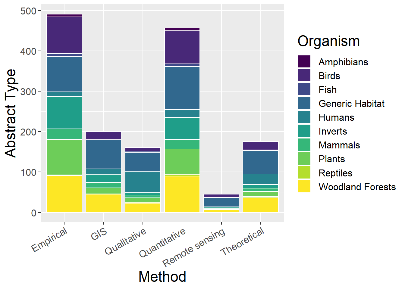

ggplot(sppCounts, aes(x=Method, y=prop, fill=Type)) + geom_bar(stat="identity", colour="white")  +
  scale_fill_viridis(discrete = TRUE) +
  theme(axis.text.x = element_text(angle = 30, hjust = 1)) +
  labs(fill="Organism", y = "Proportion", x="Method")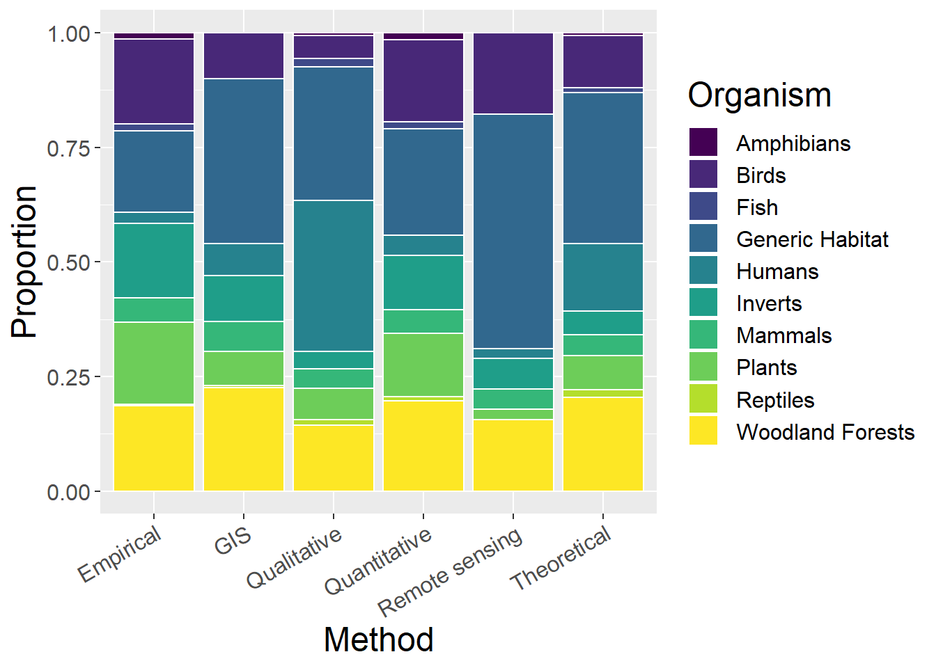

6.5 Spatial Extent

General observations:

• Theoretical studies have largely undefined extent
• No micro qualitative studies
• Very few global empirical studies, and no GIS global studies

spatialCounts <- metdata %>%
  select(Method, Micro, Mini, Local, Regional, National, Continental, Global,`Undefined Extent`) %>%
  mutate(sum = rowSums(.[2:9])) %>%
  gather(key = Type, value = count, -Method, -sum) %>%
  mutate(prop = count / sum) 

factor_order <- c('Micro', 'Mini', 'Local', 'Regional', 'National', 'Continental', 'Global','Undefined Extent')
factor_labels <- c('Micro', 'Mini', 'Local', 'Regional', 'National', 'Continental', 'Global','Undefined')

ggplot(spatialCounts, aes(x=Method, y=count, fill=factor(Type, level=factor_order))) + geom_bar(stat="identity", colour="white") +
  scale_fill_viridis(discrete = TRUE) +
  theme(axis.text.x = element_text(angle = 30, hjust = 1)) +
  labs(fill="Extent", y = "Abstract Count", x="Organism")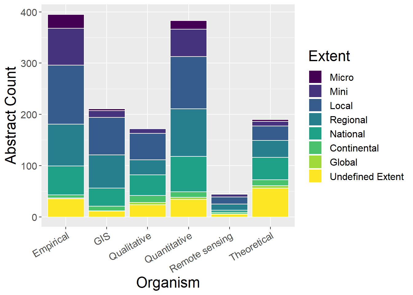

ggplot(spatialCounts, aes(x=Method, y=prop, fill=factor(Type, level=factor_order))) + geom_bar(stat="identity", colour="white")  +
  scale_fill_viridis(discrete = TRUE) +
  theme(axis.text.x = element_text(angle = 30, hjust = 1)) +
  labs(fill="Extent", y = "Proportion", x="Organism")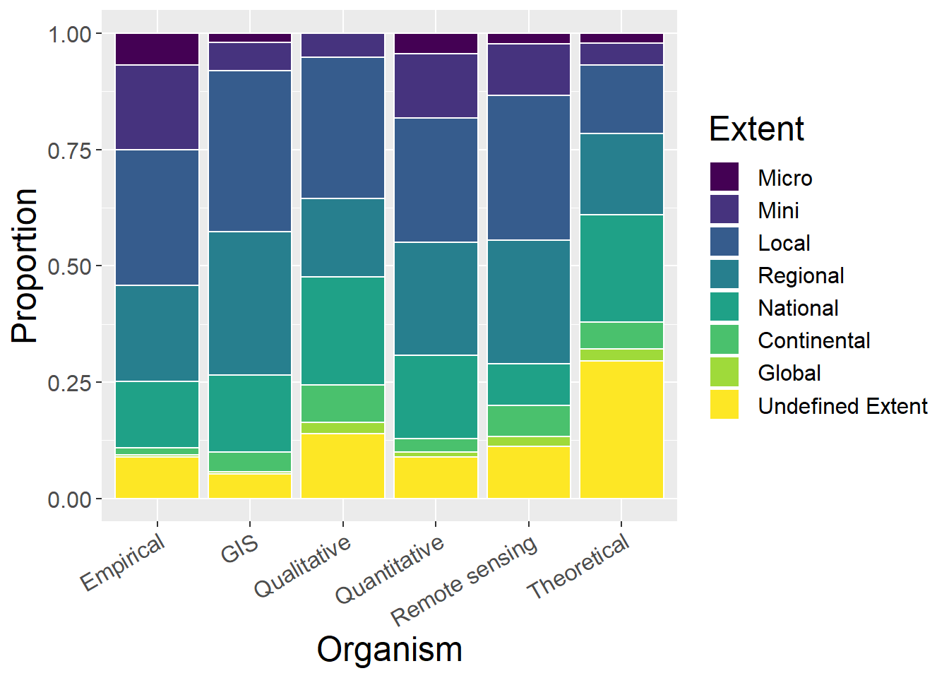

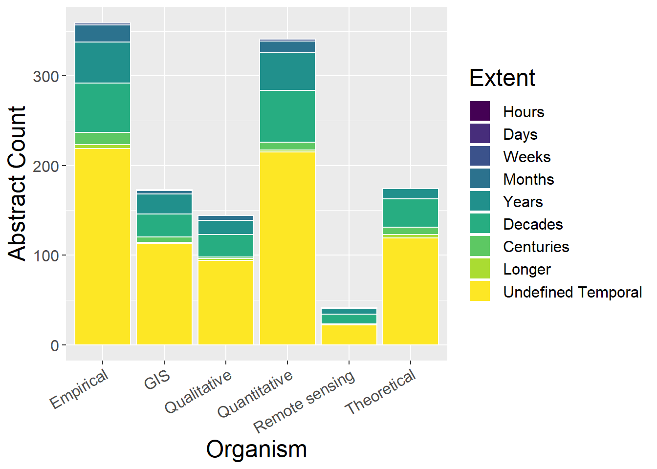
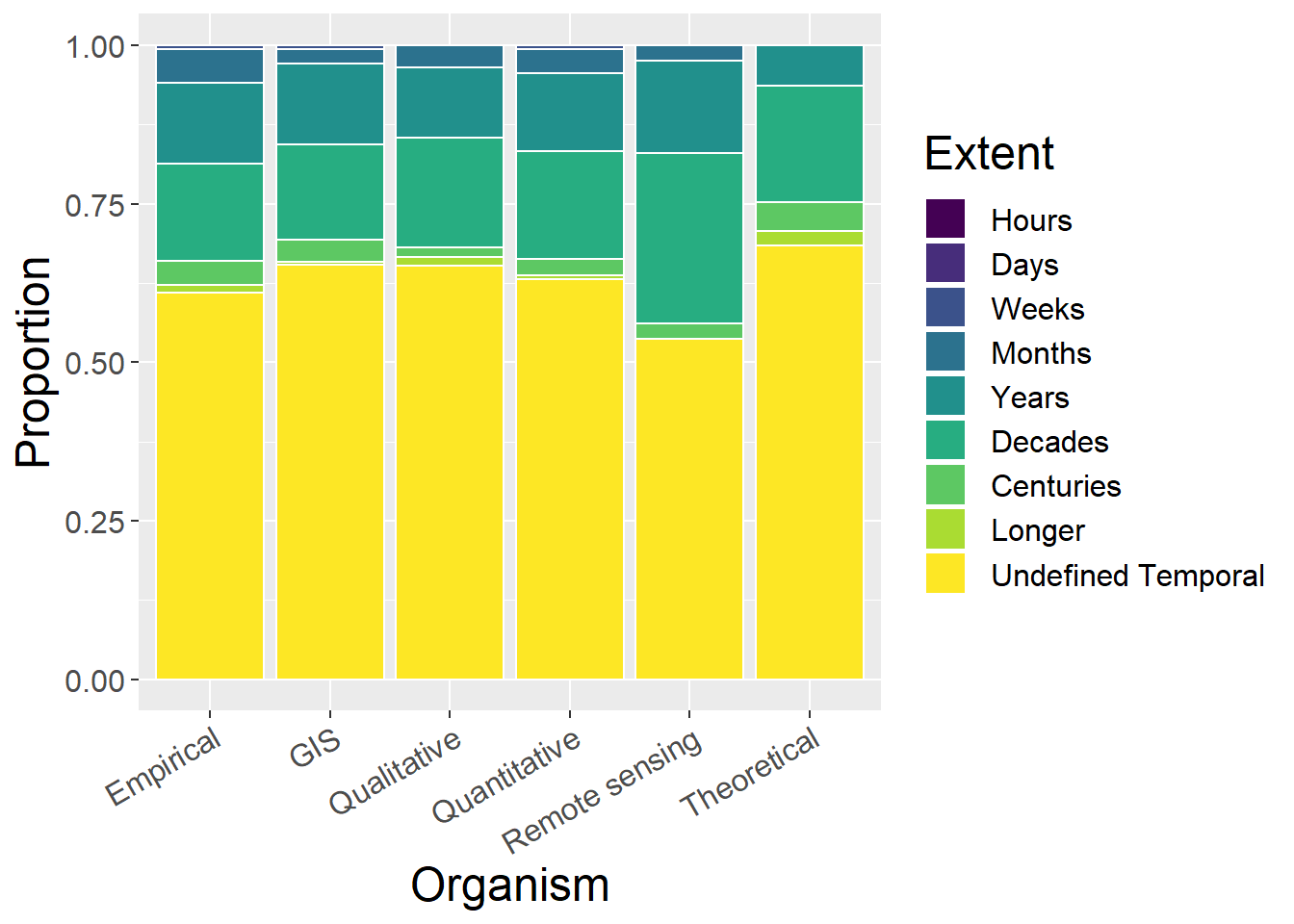
6.6 Temporal Extent

6.6.1 With undefined

General observations:

• Difficult to see much; examine without ‘undefined’

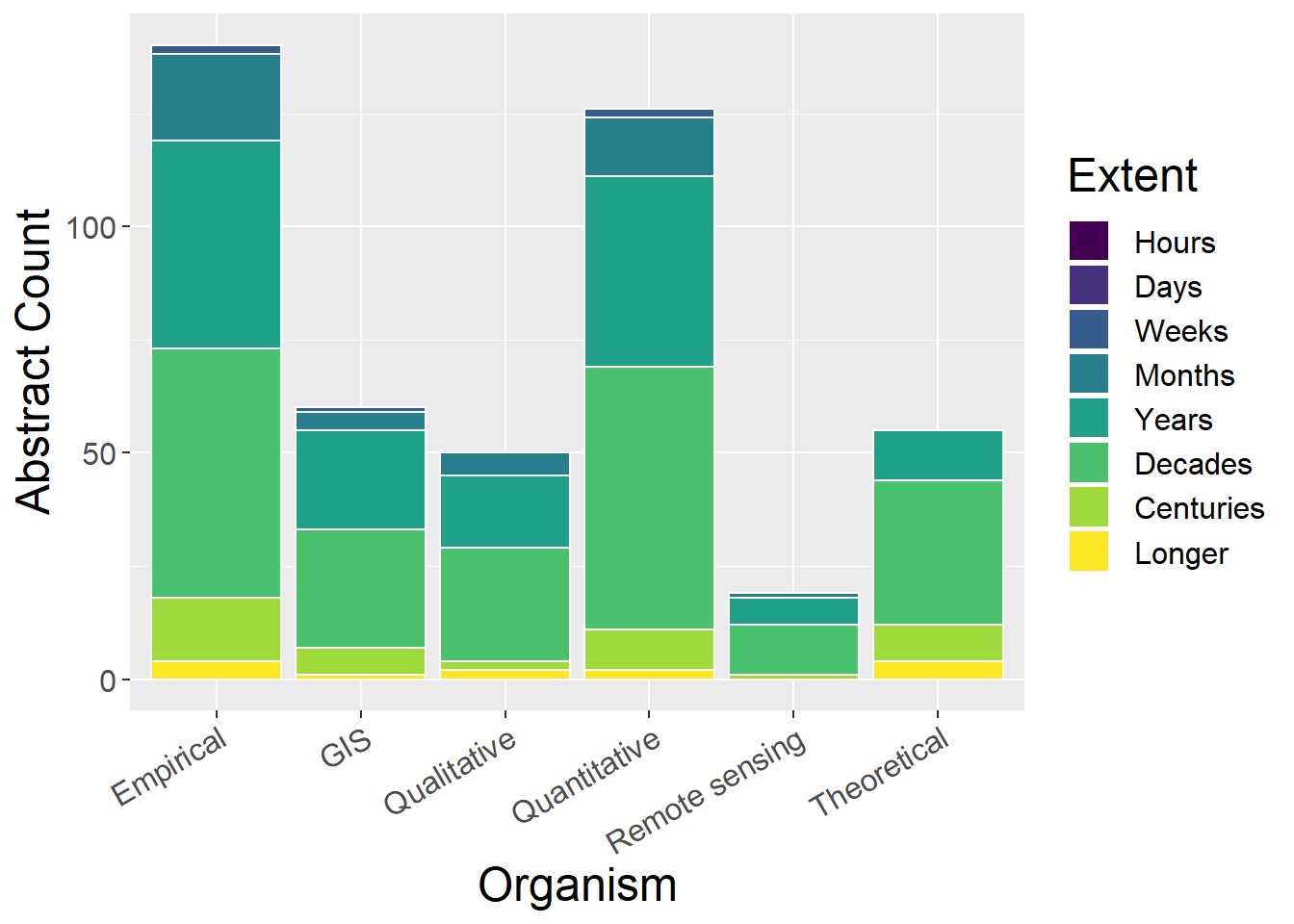
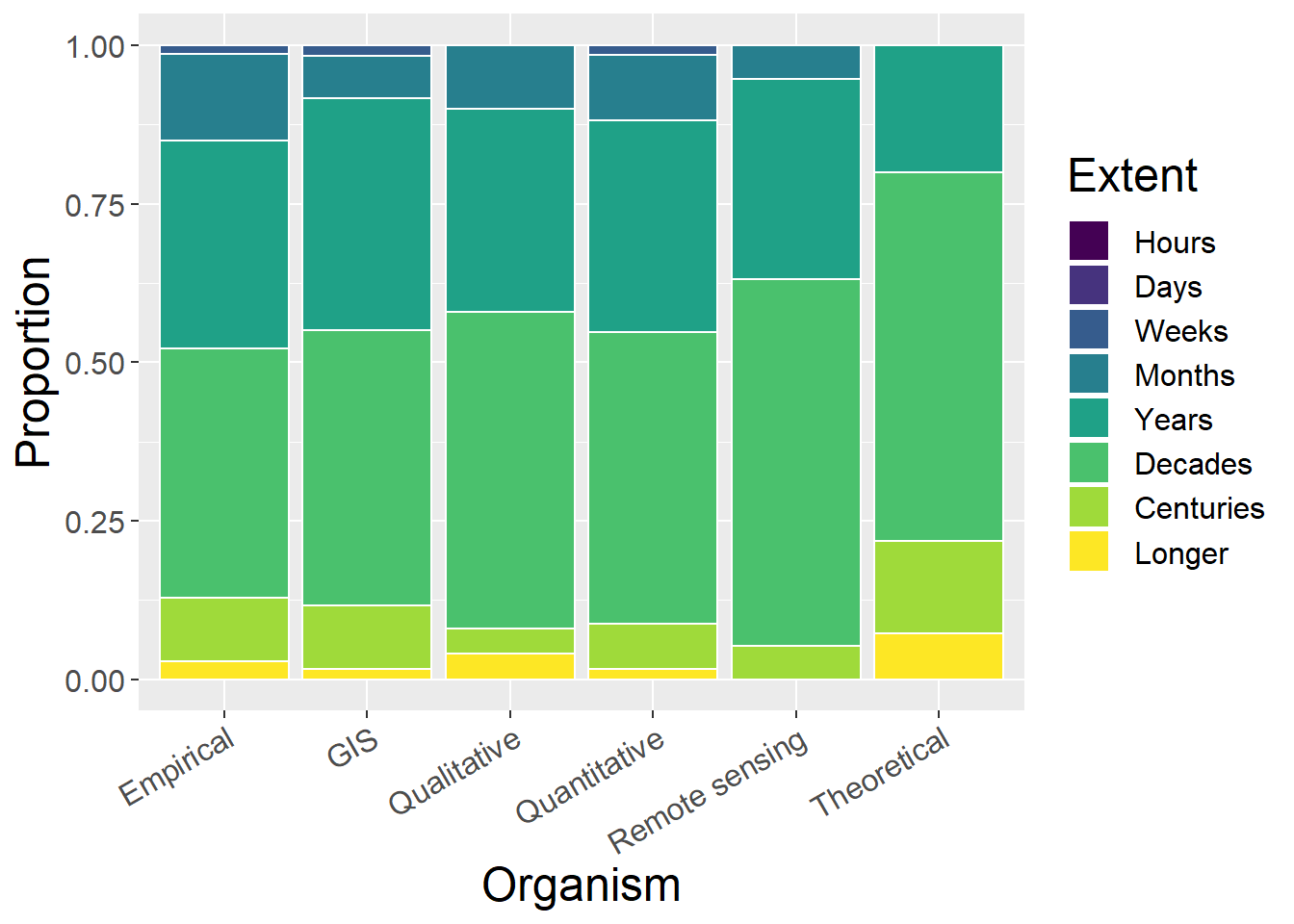
6.6.2 Without Undefined

• Theoretical studies are years or longer
• Actually, vast majority of studies are months or longer (should see this when splitting by temporal extent)

6.7 Concepts

General observations:

• Surprisingly few theoretical studies of scale and scaling?
• Relatively large number of qualitative studies are about landscape sustainability
• Relatively few empirical studies of ecosystem services
• GIS studies have largest proportion of spatial analysis and modelling (unsurprisingly)

conceptCounts <- metdata %>%
  select(Method, `PPS of landscapes`,
`Connectivity and fragmentation`, `Scale and scaling`,`Spatial analysis and modeling`,LUCC,`History and legacy`,`Climate change interactions`,`Ecosystem services`,`Landscape sustainability`,`Accuracy and uncertainty`
) %>%
  mutate(sum = rowSums(.[2:11])) %>%
  gather(key = Type, value = count, -Method, -sum) %>%
  mutate(prop = count / sum) 

ggplot(conceptCounts, aes(x=Method, y=count, fill=Type)) + geom_bar(stat="identity", colour="white") +
  scale_fill_viridis(discrete = TRUE) +
  theme(axis.text.x = element_text(angle = 30, hjust = 1)) +
  labs(fill="Concept", y = "Abstract Count", x="Organism")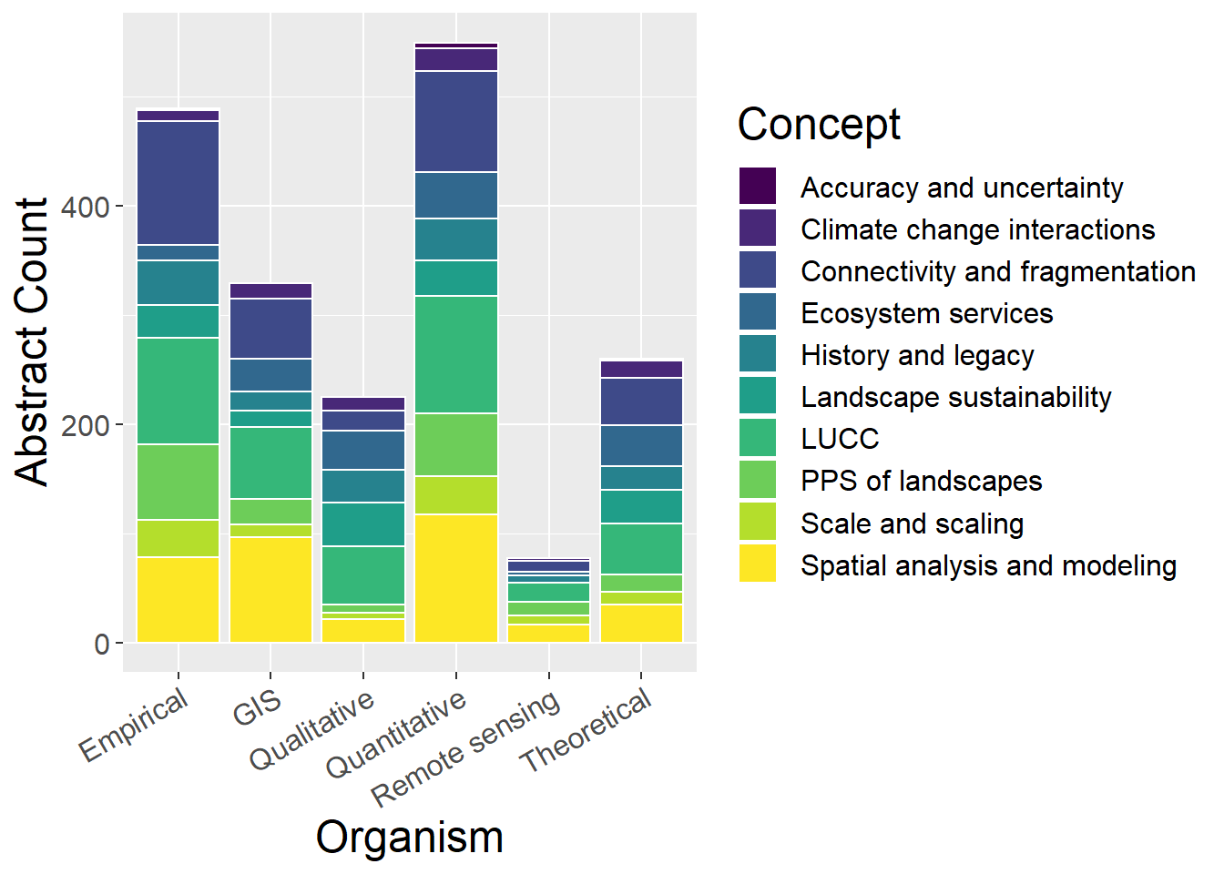

ggplot(conceptCounts, aes(x=Method, y=prop, fill=Type)) + geom_bar(stat="identity", colour="white") +
  scale_fill_viridis(discrete = TRUE) +
  theme(axis.text.x = element_text(angle = 30, hjust = 1)) +
  labs(fill="Concept", y = "Proportion", x="Organism")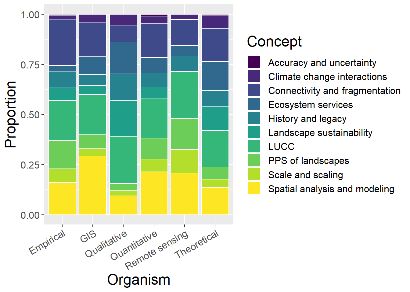

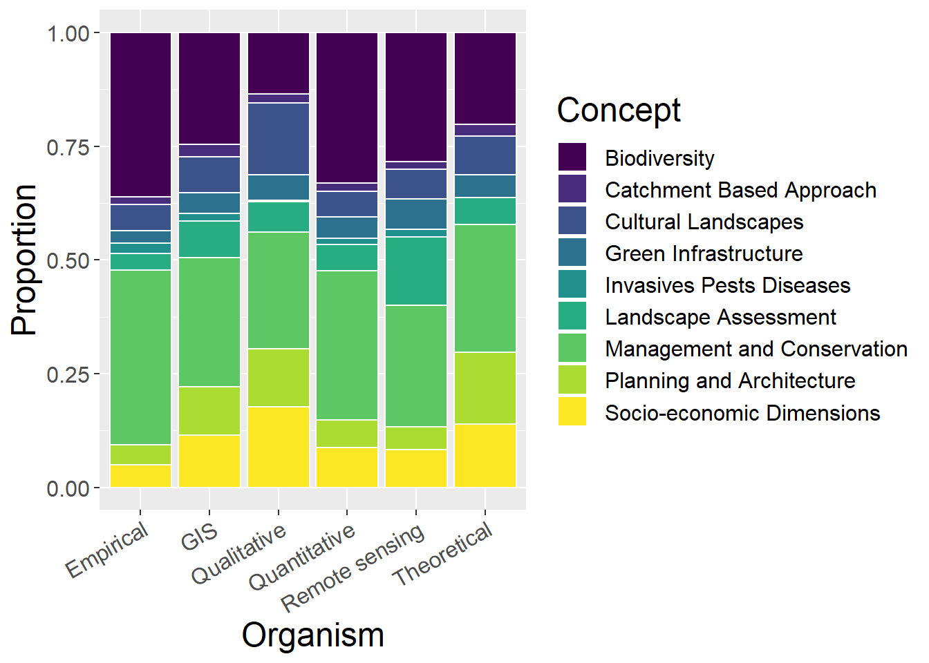
6.8 Other Concepts

General observations:

• Qualitative studies have relatively low proportion of biodiversity studies, but have relatively large proportion of socio-economic and cultural
• Theoretical studies have similar distribution to qualitative slightly more biodiversity at expense of cultural

othCCounts <- metdata %>%
  select(Method, `Green Infrastructure`,`Planning and Architecture`,`Management and Conservation`,`Cultural Landscapes`,`Socio-economic Dimensions`,Biodiversity,`Landscape Assessment`,`Catchment Based Approach`,`Invasives Pests Diseases`
) %>%
  mutate(sum = rowSums(.[2:10])) %>%
  gather(key = Type, value = count, -Method, -sum) %>%
  mutate(prop = count / sum) 

ggplot(othCCounts, aes(x=Method, y=count, fill=Type)) + geom_bar(stat="identity", colour="white") +
  scale_fill_viridis(discrete = TRUE) +
  theme(axis.text.x = element_text(angle = 30, hjust = 1)) +
  labs(fill="Concept", y = "Abstract Count", x="Organism")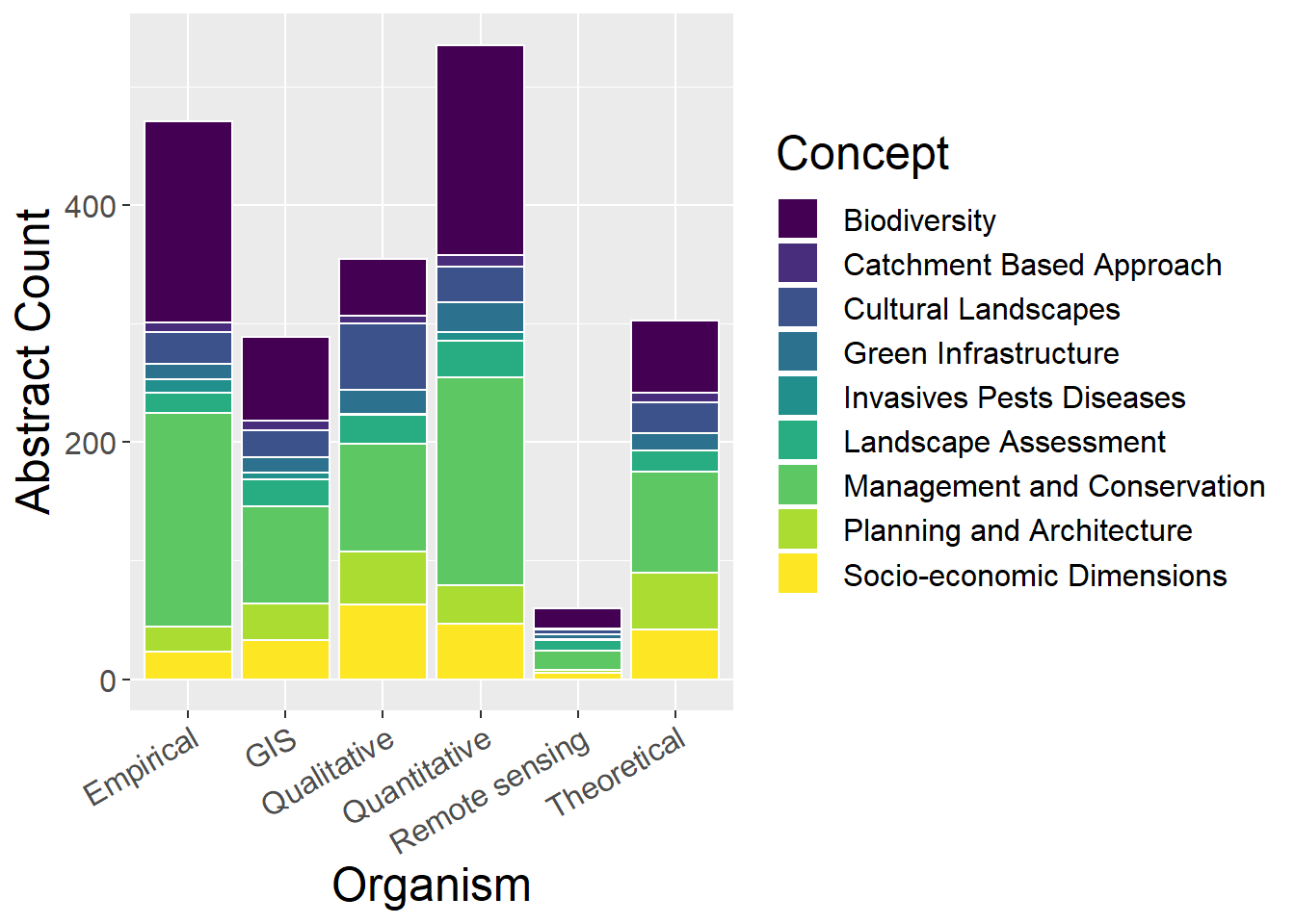

ggplot(othCCounts, aes(x=Method, y=prop, fill=Type)) + geom_bar(stat="identity", colour="white") +
  scale_fill_viridis(discrete = TRUE) +
  theme(axis.text.x = element_text(angle = 30, hjust = 1)) +
  labs(fill="Concept", y = "Proportion", x="Organism")